The original question: I’m having a debate with my wife that I think you can help us resolve. We have a swimming pool in our back yard. It has an electric heater, which we set to keep the pool water at 85 degrees Fahrenheit. We’re going to be away for three days. My wife says we should turn the heater off while we’re away to save energy. I say that it takes less energy to maintain the pool at 85 while we’re away then to let it drop about ten degrees (summer evenings can get quite cool where we live in upstate New York) and then use the heater to restore 85. Who’s right? And what variables are relevant to the calculation? The average temperature for the three days? The volume of the pool? The efficiency of the heater?
Physicist: The correct answer is always to leave the heater off for as long as possible, as often as possible. The one and only gain from leaving a pool heater on is that it will be warm when you get in. The same is true of all heaters (pool, car, space, whatever).
You can gain a lot of intuition for how heat flows from place to place by imagining it as a bunch of “heat beads”, randomly skittering through matter. Each bead rolls independently from place to place, continuously changing direction, and the more beads there are in a given place, the hotter it is.
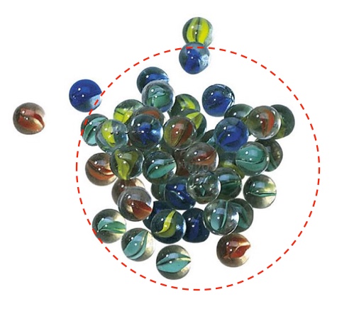
If all of these marbles started to randomly roll around, more would roll out of the circle than roll in. Heat flow works the same way: hotter to cooler.
Although heat definitely does not take the form of discrete chunks of energy meandering about, this metaphor is remarkably good. You can actually derive useful math from it, which is a damn sight better than most science metaphors (E.g., “space is like a rubber sheet” is not useful for actual astrophysicists). In very much the same way that a concentrated collection of beads will spread themselves uniformly, hot things will lose heat energy to the surrounding cooler environment. If the temperature of the pool and the air above it are equal, then the amount of heat that flows out of the pool is equal to the amount that flows in. But if the pool is hotter, then more “beads” will randomly roll out than randomly roll in.
A difference in temperature leads to a net flow of heat energy. In fact, the relationship is as simple as it can (reasonably) get: the rate of heat transfer is proportional to the difference in temperature. So, if the surrounding air is 60°, then an 80° pool will shed heat energy twice as fast as a 70° pool. This is why coffee/tea/soup will be hot for a little while, but tepid for a long time; it cools faster when it’s hotter.

In a holy bucket, the higher the water level, the faster the water flows out. Differences in temperature work the same way. The greater the difference in temperature, the faster the heat flows out.
Ultimately, the amount of energy that a heater puts into the pool is equal to the heat lost from the pool. Since you lose more heat energy from a hot pool than from a cool pool, the most efficient thing you can do is keep the temperature as low as possible for as long as possible. The most energy efficient thing to do is always to turn off the heater. The only reason to keep it on is so that you don’t have to wait for the water to warm up before you use it.
It seems as though a bunch of water is a good place to store heat energy, but the more time something spends being hot, the more energy it drains into everything around it.
Answer Gravy: This gravy is just to delve into why picturing heat flow in terms of the random motion of hypothetical particles is a good idea. It’s well worth taking a stroll through statistical mechanics every now and again.
The diffusion of heat is governed, not surprisingly, by the “diffusion equation”.

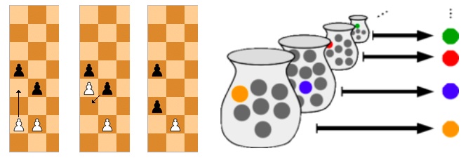
The same equation describes the random motion of particles. If ρ(x,t) is the amount of heat at any given location, x, and time, t, then the diffusion equation tells you how that heat will change over time. On the other hand, if ρ is either the density of “beads” or the probability of finding a bead at a particular place (if the movement of the beads is independent, then these two situations are interchangeable), then once again the diffusion equation describes how the bead density changes over time. This is why the idea of “heat beads” is a useful intuition to use; the same math that describes the random motion of particles also describes how heat spreads through materials.
In one of his terribly clever 1905 papers, Einstein described how the random motion of individual atoms gives rise to diffusion. The idea is to look at ρ(x,t) and then figure out ρ(x,t+τ), which is what it will be one small time step, τ, later. If you put a particle down somewhere, wait τ seconds and check where it is over and over, then you can figure out the probability of the particle drifting some distance, ε. Just to give it a name, call that probability ϕ(ε).
ϕ(ε) is a recipe for figuring out how ρ(x,t) changes over time. The probability that the particle will end up at, say, x=5 is equal to the probability that it was at x=3 times ϕ(2) plus the probability that it was at x=1 times ϕ(4) plus the probability that it was at x=8 times ϕ(-3) and so on, for every number. Adding up the probabilities from every possible starting position is the sort of thing integrals were made for:
=\int\rho(x+\epsilon,t)\phi(-\epsilon)d\epsilon")
So far this is standard probability fare. Einstein’s cute trick was to say “Listen, I don’t know what ϕ(ε) is, but I know it’s symmetrical and it’s some kind of probability thing, which is pretty good, amirite?”.
ρ(x,t) varies smoothly (particles don’t teleport) which means ρ(x,t) can be expanded into a Taylor series in x or t. That looks like:
=\rho(x,t)+\tau\frac{d}{dt}\rho(x,t)+\frac{\tau^2}{2}\frac{d^2}{dt^2}\rho(x,t)+\ldots")
and
=\rho(x,t)+\epsilon\frac{d}{dx}\rho(x,t)+\frac{\epsilon^2}{2}\frac{d^2}{dx^2}\rho(x,t)+\ldots")
where “…” are the higher order terms, that are all very small as long as τ and ε are small. Plugging the expansion of ρ(x+ε,t) into \phi(-\epsilon)d\epsilon")
![\begin{array}{ll}&\int\left[\rho(x,t)+\epsilon\frac{d}{dx}\rho(x,t)+\frac{\epsilon^2}{2}\frac{d^2}{dx^2}\rho(x,t)+\ldots\right]\phi(-\epsilon)d\epsilon\\[2mm]=&\rho(x,t)\int\phi(-\epsilon)d\epsilon+\frac{d}{dx}\rho(x,t)\int\epsilon\phi(-\epsilon)d\epsilon+\frac{d^2}{dx^2}\rho(x,t)\int\frac{\epsilon^2}{2}\phi(-\epsilon)d\epsilon+\ldots\\[2mm]=&\rho(x,t)+\left[\int\frac{\epsilon^2}{2}\phi(-\epsilon)d\epsilon\right]\frac{d^2}{dx^2}\rho(x,t)+\ldots\end{array}](https://s0.wp.com/latex.php?latex=%5Cbegin%7Barray%7D%7Bll%7D%26%5Cint%5Cleft%5B%5Crho%28x%2Ct%29%2B%5Cepsilon%5Cfrac%7Bd%7D%7Bdx%7D%5Crho%28x%2Ct%29%2B%5Cfrac%7B%5Cepsilon%5E2%7D%7B2%7D%5Cfrac%7Bd%5E2%7D%7Bdx%5E2%7D%5Crho%28x%2Ct%29%2B%5Cldots%5Cright%5D%5Cphi%28-%5Cepsilon%29d%5Cepsilon%5C%5C%5B2mm%5D%3D%26%5Crho%28x%2Ct%29%5Cint%5Cphi%28-%5Cepsilon%29d%5Cepsilon%2B%5Cfrac%7Bd%7D%7Bdx%7D%5Crho%28x%2Ct%29%5Cint%5Cepsilon%5Cphi%28-%5Cepsilon%29d%5Cepsilon%2B%5Cfrac%7Bd%5E2%7D%7Bdx%5E2%7D%5Crho%28x%2Ct%29%5Cint%5Cfrac%7B%5Cepsilon%5E2%7D%7B2%7D%5Cphi%28-%5Cepsilon%29d%5Cepsilon%2B%5Cldots%5C%5C%5B2mm%5D%3D%26%5Crho%28x%2Ct%29%2B%5Cleft%5B%5Cint%5Cfrac%7B%5Cepsilon%5E2%7D%7B2%7D%5Cphi%28-%5Cepsilon%29d%5Cepsilon%5Cright%5D%5Cfrac%7Bd%5E2%7D%7Bdx%5E2%7D%5Crho%28x%2Ct%29%2B%5Cldots%5Cend%7Barray%7D&bg=ffffff&fg=000000&s=0 "\begin{array}{ll}&\int\left[\rho(x,t)+\epsilon\frac{d}{dx}\rho(x,t)+\frac{\epsilon^2}{2}\frac{d^2}{dx^2}\rho(x,t)+\ldots\right]\phi(-\epsilon)d\epsilon\\[2mm]=&\rho(x,t)\int\phi(-\epsilon)d\epsilon+\frac{d}{dx}\rho(x,t)\int\epsilon\phi(-\epsilon)d\epsilon+\frac{d^2}{dx^2}\rho(x,t)\int\frac{\epsilon^2}{2}\phi(-\epsilon)d\epsilon+\ldots\\[2mm]=&\rho(x,t)+\left[\int\frac{\epsilon^2}{2}\phi(-\epsilon)d\epsilon\right]\frac{d^2}{dx^2}\rho(x,t)+\ldots\end{array}")
Einstein’s cute tricks both showed up in that last line. d\epsilon=0")
d\epsilon=1")
So,
![\begin{array}{rcl}\rho(x,t)+\tau\frac{d}{dt}\rho(x,t)+\ldots&=&\rho(x,t)+\left[\int\frac{\epsilon^2}{2}\phi(-\epsilon)d\epsilon\right]\frac{d^2}{dx^2}\rho(x,t)+\ldots\\[2mm]\tau\frac{d}{dt}\rho(x,t)&=&\left[\int\frac{\epsilon^2}{2}\phi(-\epsilon)d\epsilon\right]\frac{d^2}{dx^2}\rho(x,t)+\ldots\\[2mm]\frac{d}{dt}\rho(x,t)&=&\left[\int\frac{\epsilon^2}{2\tau}\phi(-\epsilon)d\epsilon\right]\frac{d^2}{dx^2}\rho(x,t)+\ldots\\[2mm]\end{array}](https://s0.wp.com/latex.php?latex=%5Cbegin%7Barray%7D%7Brcl%7D%5Crho%28x%2Ct%29%2B%5Ctau%5Cfrac%7Bd%7D%7Bdt%7D%5Crho%28x%2Ct%29%2B%5Cldots%26%3D%26%5Crho%28x%2Ct%29%2B%5Cleft%5B%5Cint%5Cfrac%7B%5Cepsilon%5E2%7D%7B2%7D%5Cphi%28-%5Cepsilon%29d%5Cepsilon%5Cright%5D%5Cfrac%7Bd%5E2%7D%7Bdx%5E2%7D%5Crho%28x%2Ct%29%2B%5Cldots%5C%5C%5B2mm%5D%5Ctau%5Cfrac%7Bd%7D%7Bdt%7D%5Crho%28x%2Ct%29%26%3D%26%5Cleft%5B%5Cint%5Cfrac%7B%5Cepsilon%5E2%7D%7B2%7D%5Cphi%28-%5Cepsilon%29d%5Cepsilon%5Cright%5D%5Cfrac%7Bd%5E2%7D%7Bdx%5E2%7D%5Crho%28x%2Ct%29%2B%5Cldots%5C%5C%5B2mm%5D%5Cfrac%7Bd%7D%7Bdt%7D%5Crho%28x%2Ct%29%26%3D%26%5Cleft%5B%5Cint%5Cfrac%7B%5Cepsilon%5E2%7D%7B2%5Ctau%7D%5Cphi%28-%5Cepsilon%29d%5Cepsilon%5Cright%5D%5Cfrac%7Bd%5E2%7D%7Bdx%5E2%7D%5Crho%28x%2Ct%29%2B%5Cldots%5C%5C%5B2mm%5D%5Cend%7Barray%7D&bg=ffffff&fg=000000&s=0 "\begin{array}{rcl}\rho(x,t)+\tau\frac{d}{dt}\rho(x,t)+\ldots&=&\rho(x,t)+\left[\int\frac{\epsilon^2}{2}\phi(-\epsilon)d\epsilon\right]\frac{d^2}{dx^2}\rho(x,t)+\ldots\\[2mm]\tau\frac{d}{dt}\rho(x,t)&=&\left[\int\frac{\epsilon^2}{2}\phi(-\epsilon)d\epsilon\right]\frac{d^2}{dx^2}\rho(x,t)+\ldots\\[2mm]\frac{d}{dt}\rho(x,t)&=&\left[\int\frac{\epsilon^2}{2\tau}\phi(-\epsilon)d\epsilon\right]\frac{d^2}{dx^2}\rho(x,t)+\ldots\\[2mm]\end{array}")
To make the jump from discrete time steps to continuous time, we just let the time step, τ, shrink to zero (which also forces the distances involved, ε, to shrink since there’s less time to get anywhere). As τ and ε get very small, the higher order terms dwindle away and we’re left with ![\frac{d}{dt}\rho(x,t)=\left[\int\frac{\epsilon^2}{2\tau}\phi(-\epsilon)d\epsilon\right]\frac{d^2}{dx^2}\rho(x,t)](https://s0.wp.com/latex.php?latex=%5Cfrac%7Bd%7D%7Bdt%7D%5Crho%28x%2Ct%29%3D%5Cleft%5B%5Cint%5Cfrac%7B%5Cepsilon%5E2%7D%7B2%5Ctau%7D%5Cphi%28-%5Cepsilon%29d%5Cepsilon%5Cright%5D%5Cfrac%7Bd%5E2%7D%7Bdx%5E2%7D%5Crho%28x%2Ct%29&bg=ffffff&fg=000000&s=0 "\frac{d}{dt}\rho(x,t)=\left[\int\frac{\epsilon^2}{2\tau}\phi(-\epsilon)d\epsilon\right]\frac{d^2}{dx^2}\rho(x,t)")
d\epsilon")
The second derivative, 
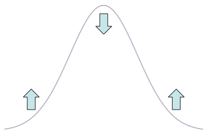
The diffusion equation dictates that if the graph is concave down, the density drops and if the graph is concave up, the density increases.
This is a very long-winded way of saying “think of heat as randomly moving particles, because the math is the same”. But again, heat isn’t actually particles, it’s just that picturing it as such leads to useful insights. While the equation and the intuition are straight forward, actually solving the diffusion equation in almost any real world scenario is a huge pain.
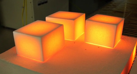
The corners cool off faster because there are more opportunities for “heat beads” to fall out of the material there. Although this is exactly what the diffusion equation predicts, actually doing the math by hand is difficult.
It’s all well and good to talk about how heat beads randomly walk around inside of a material, but if that material isn’t uniform or has an edge, then suddenly the math gets remarkably nasty. Fortunately, if all you’re worried about is whether or not you should leave your heater on, then you’re probably not sweating the calculus.
The shuttle tile photo is from here.


 into the thin lens equation and you find that
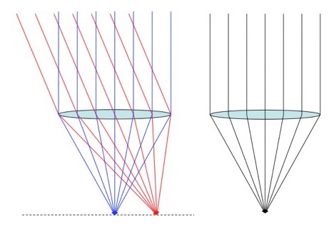
  , and so di=f. In other words, the Sun, and everything else “at infinity”, will be in focus f away from the lens. This coincides with the definition of the focal length, since light from a source at infinity is always parallel. That should jive with your our experience: if you look at a light ten feet away and you step back and forth, the angle to the light changes, but if you look at the Sun (don’t) and step back and forth, the angle to the Sun stays the same.
 . As with the resolution to
  isn’t. By measuring the Sun’s apparent size in the sky, it’s easy to figure out that it’s 110 times farther away than it is big. The same thing, very coincidentally, is true of the Moon; it is 110 Moon-diameters away from Earth. Mathematically speaking,
  .
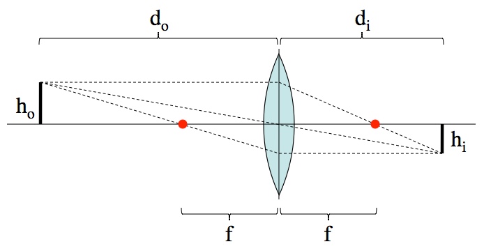
. , into play. That was intentional; pretending there’s an issue heightens drama. Solving for the image size, hi, and plugging in what we already know,
 . This ultimately comes down to the fact that the Sun is really far away, and 110 times smaller than it is distant.
 . Rearranging this to put the h’s and d’s on opposite sides produces the magnification equation,
  . Easy!
![\begin{array}{rcl}\frac{h_o}{f}&=&\frac{h_o+h_i}{d_i}\\[2mm]\frac{h_o}{f}&=&\frac{h_o}{d_i}+\frac{h_i}{d_i}\\[2mm]\frac{h_o}{f}&=&\frac{h_o}{d_i}+\frac{h_o}{d_o}\\[2mm]\frac{1}{f}&=&\frac{1}{d_i}+\frac{1}{d_o}\end{array}](https://s0.wp.com/latex.php?latex=%5Cbegin%7Barray%7D%7Brcl%7D%5Cfrac%7Bh_o%7D%7Bf%7D%26%3D%26%5Cfrac%7Bh_o%2Bh_i%7D%7Bd_i%7D%5C%5C%5B2mm%5D%5Cfrac%7Bh_o%7D%7Bf%7D%26%3D%26%5Cfrac%7Bh_o%7D%7Bd_i%7D%2B%5Cfrac%7Bh_i%7D%7Bd_i%7D%5C%5C%5B2mm%5D%5Cfrac%7Bh_o%7D%7Bf%7D%26%3D%26%5Cfrac%7Bh_o%7D%7Bd_i%7D%2B%5Cfrac%7Bh_o%7D%7Bd_o%7D%5C%5C%5B2mm%5D%5Cfrac%7B1%7D%7Bf%7D%26%3D%26%5Cfrac%7B1%7D%7Bd_i%7D%2B%5Cfrac%7B1%7D%7Bd_o%7D%5Cend%7Barray%7D&bg=ffffff&fg=000000&s=0 "\begin{array}{rcl}\frac{h_o}{f}&=&\frac{h_o+h_i}{d_i}\\[2mm]\frac{h_o}{f}&=&\frac{h_o}{d_i}+\frac{h_i}{d_i}\\[2mm]\frac{h_o}{f}&=&\frac{h_o}{d_i}+\frac{h_o}{d_o}\\[2mm]\frac{1}{f}&=&\frac{1}{d_i}+\frac{1}{d_o}\end{array}")

 , which can be done using the
 \pm\sqrt{(2)^2-4(1)(-3)}}{2(1)}=\frac{-2\pm4}{2}=-3\,or\,1")
 (and who doesn’t?) there is literally no way to find an expression for the exact answers.
 (3.14159…)
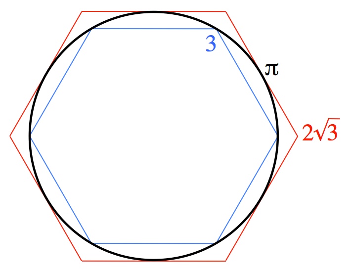
 and
and  and produces the perimeters for polygons with twice the numbers of sides,
  and
and  . Here’s the method:
 and
and  , and doubling the number of sides 4 times Archie found that for inscribed and circumscribed
  and
and  . In other words, he managed to nail down
  .
.\approx\pi-\frac{\pi^3}{6}\frac{1}{n^2}") and
and \approx\pi+\frac{\pi^3}{3}\frac{1}{n^2}") . Every time you double n the errors,
. Every time you double n the errors,  and
and  , get four times as small (because
  ), which translates to very roughly one new decimal place every two iterations.
  and call that number k. If you do this many times, you’ll find that
  .
.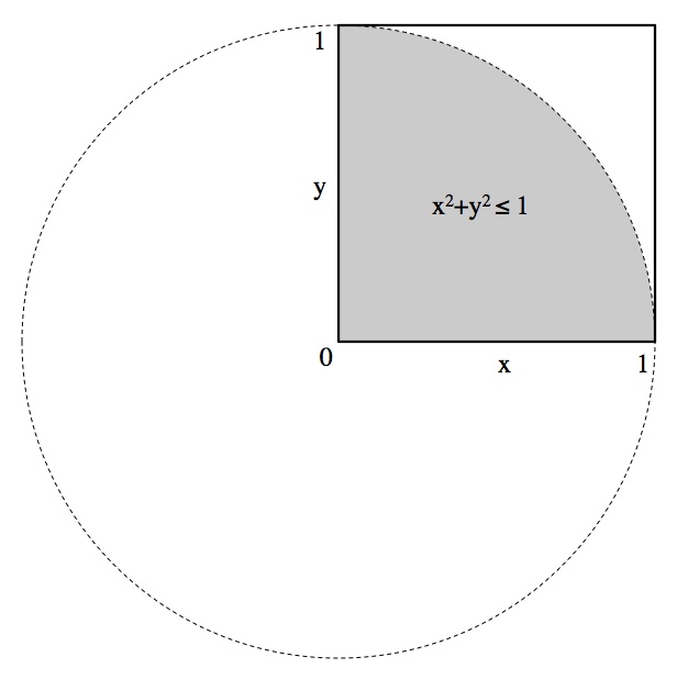
 , since that’s the probability of randomly falling in the grey region in the picture above. This numerical method is even slower than Archimedes’ not-particularly-speedy trick. According to the
  of
of  , such that
 =0") . The whole idea is that, assuming the function is
. The whole idea is that, assuming the function is 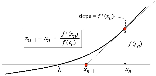
") is the slope at the point
is the slope at the point )") . Considering the picture above, that same slope is given by the rise,
. Considering the picture above, that same slope is given by the rise, ") , over the run,
, over the run,  . In other words
 =\frac{f(x_n)}{x_n-x_{n+1}}") which can be solved for
which can be solved for  :
:}{f^\prime(x_n)}")
 , you can find another point that’s closer to the true solution,
 \approx0") , then
, then  . That’s good: when you’ve got the right answer, you don’t want your approximation to change.
 . With this tiny equation in hand you can quickly find
  . With
  and so on. Although it can take a few iterations for it to settle down, each new
 ") for x. Never mind why. There is no analytical solution (this comes up a lot when you mix polynomials, like x, or trig functions or logs or just about anything). The correct answer starts with
for x. Never mind why. There is no analytical solution (this comes up a lot when you mix polynomials, like x, or trig functions or logs or just about anything). The correct answer starts with 
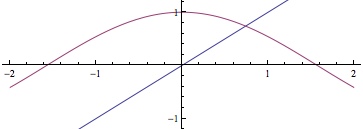
=\cos(x)-x=0") . The derivative is
. The derivative is =-\sin(x)-1") and therefore:
and therefore:}{f^\prime\left(x_n\right)}=x_n+\frac{\cos\left(x_n\right)-x_n}{\sin\left(x_n\right)+1}")
 . Plug that in and you find that:
-x_0}{\sin\left(x_0\right)+1}=3+\frac{\cos\left(3\right)-3}{\sin\left(3\right)+1}=-0.496558178297331398840279")

 jump around a bit. Sometimes Newton’s method does this forever (try
  ) in which case: try something else or make a new guess. It’s not until
  that Newton’s method starts to really zero in on the solution. Notice that (starting at
^2=0.0001") . In other words, the number of digits you can be confident in doubles every time.
. In other words, the number of digits you can be confident in doubles every time.") and
and }{f^\prime\left(x_n\right)}") .
.![\begin{array}{rcl} 0&=&f(\lambda) \\[2mm] 0&=&f(x_n+(\lambda-x_n)) \\[2mm] 0&=&f(x_n)+f^\prime(x_n)\left(\lambda-x_n\right)+\frac{1}{2}f^{\prime\prime}(x_n)\left(\lambda-x_n\right)^2+\ldots \\[2mm] 0&=&\frac{f\left(x_n\right)}{f^\prime\left(x_n\right)}+\left(\lambda-x_n\right)+\frac{f^{\prime\prime}(x_n)}{2f^\prime\left(x_n\right)}\left(\lambda-x_n\right)^2+\ldots \\[2mm] 0&=&\lambda-\left(x_n-\frac{f\left(x_n\right)}{f^\prime\left(x_n\right)}\right)+\frac{f^{\prime\prime}(x_n)}{2f^\prime\left(x_n\right)}\left(\lambda-x_n\right)^2+\ldots \\[2mm] 0&=&\lambda-x_{n+1}+\frac{f^{\prime\prime}(x_n)}{2f^\prime\left(x_n\right)}\left(\lambda-x_n\right)^2+\ldots \\[2mm] \lambda-x_{n+1}&=&-\frac{f^{\prime\prime}(x_n)}{2f^\prime\left(x_n\right)}\left(\lambda-x_n\right)^2+\ldots \end{array}](http://s0.wp.com/latex.php?latex=%5Cbegin%7Barray%7D%7Brcl%7D++0%26%3D%26f%28%5Clambda%29+%5C%5C%5B2mm%5D++0%26%3D%26f%28x_n%2B%28%5Clambda-x_n%29%29+%5C%5C%5B2mm%5D++0%26%3D%26f%28x_n%29%2Bf%5E%5Cprime%28x_n%29%5Cleft%28%5Clambda-x_n%5Cright%29%2B%5Cfrac%7B1%7D%7B2%7Df%5E%7B%5Cprime%5Cprime%7D%28x_n%29%5Cleft%28%5Clambda-x_n%5Cright%29%5E2%2B%5Cldots+%5C%5C%5B2mm%5D++0%26%3D%26%5Cfrac%7Bf%5Cleft%28x_n%5Cright%29%7D%7Bf%5E%5Cprime%5Cleft%28x_n%5Cright%29%7D%2B%5Cleft%28%5Clambda-x_n%5Cright%29%2B%5Cfrac%7Bf%5E%7B%5Cprime%5Cprime%7D%28x_n%29%7D%7B2f%5E%5Cprime%5Cleft%28x_n%5Cright%29%7D%5Cleft%28%5Clambda-x_n%5Cright%29%5E2%2B%5Cldots+%5C%5C%5B2mm%5D++0%26%3D%26%5Clambda-%5Cleft%28x_n-%5Cfrac%7Bf%5Cleft%28x_n%5Cright%29%7D%7Bf%5E%5Cprime%5Cleft%28x_n%5Cright%29%7D%5Cright%29%2B%5Cfrac%7Bf%5E%7B%5Cprime%5Cprime%7D%28x_n%29%7D%7B2f%5E%5Cprime%5Cleft%28x_n%5Cright%29%7D%5Cleft%28%5Clambda-x_n%5Cright%29%5E2%2B%5Cldots+%5C%5C%5B2mm%5D++0%26%3D%26%5Clambda-x_%7Bn%2B1%7D%2B%5Cfrac%7Bf%5E%7B%5Cprime%5Cprime%7D%28x_n%29%7D%7B2f%5E%5Cprime%5Cleft%28x_n%5Cright%29%7D%5Cleft%28%5Clambda-x_n%5Cright%29%5E2%2B%5Cldots+%5C%5C%5B2mm%5D++%5Clambda-x_%7Bn%2B1%7D%26%3D%26-%5Cfrac%7Bf%5E%7B%5Cprime%5Cprime%7D%28x_n%29%7D%7B2f%5E%5Cprime%5Cleft%28x_n%5Cright%29%7D%5Cleft%28%5Clambda-x_n%5Cright%29%5E2%2B%5Cldots++%5Cend%7Barray%7D&bg=ffffff&fg=000&s=0 "\begin{array}{rcl} 0&=&f(\lambda) \\[2mm] 0&=&f(x_n+(\lambda-x_n)) \\[2mm] 0&=&f(x_n)+f^\prime(x_n)\left(\lambda-x_n\right)+\frac{1}{2}f^{\prime\prime}(x_n)\left(\lambda-x_n\right)^2+\ldots \\[2mm] 0&=&\frac{f\left(x_n\right)}{f^\prime\left(x_n\right)}+\left(\lambda-x_n\right)+\frac{f^{\prime\prime}(x_n)}{2f^\prime\left(x_n\right)}\left(\lambda-x_n\right)^2+\ldots \\[2mm] 0&=&\lambda-\left(x_n-\frac{f\left(x_n\right)}{f^\prime\left(x_n\right)}\right)+\frac{f^{\prime\prime}(x_n)}{2f^\prime\left(x_n\right)}\left(\lambda-x_n\right)^2+\ldots \\[2mm] 0&=&\lambda-x_{n+1}+\frac{f^{\prime\prime}(x_n)}{2f^\prime\left(x_n\right)}\left(\lambda-x_n\right)^2+\ldots \\[2mm] \lambda-x_{n+1}&=&-\frac{f^{\prime\prime}(x_n)}{2f^\prime\left(x_n\right)}\left(\lambda-x_n\right)^2+\ldots \end{array}")
^2") as
as }{2f^\prime\left(x_n\right)}") becomes effectively equal to
becomes effectively equal to }{2f^\prime\left(\lambda\right)}") . Therefore
. Therefore ^2") and that’s what quadratic convergence is. Note that this only works when you’re zeroing in; far away from the correct answer Newton’s method can really bounce around.
and that’s what quadratic convergence is. Note that this only works when you’re zeroing in; far away from the correct answer Newton’s method can really bounce around.
 . More than merely a statement of fact, mathematical expressions like this allow us to describe/predict precisely how things physically behave. We can
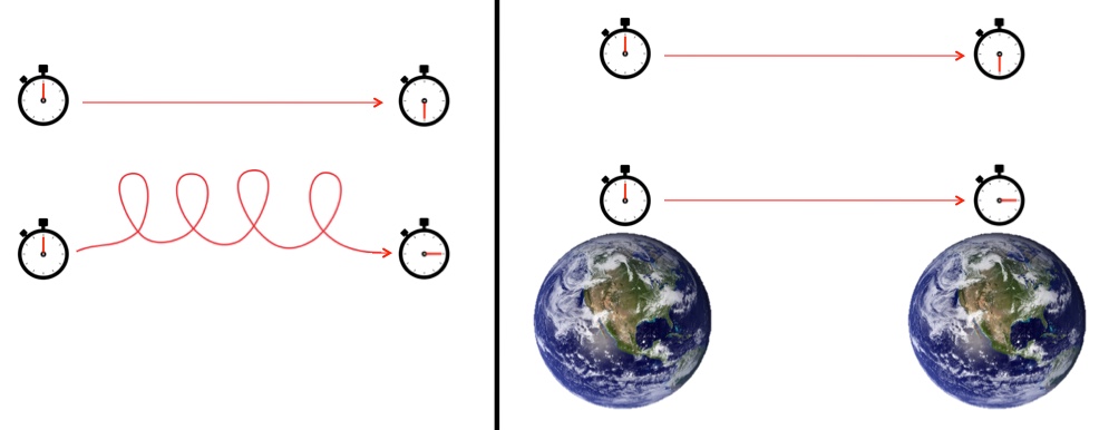
 amount of time and the stationary clock experiences
  amount of time, then
 ^2}") (which you’ll notice is always less than t) where v is the speed of the traveling clock and c is the speed of light. The ratio between these two times is called “gamma”,
(which you’ll notice is always less than t) where v is the speed of the traveling clock and c is the speed of light. The ratio between these two times is called “gamma”, ^2}}") , which is a useful piece of math to be aware of.
, which is a useful piece of math to be aware of. }{c}\right)^2}\,dt=\int_0^t \frac{dt}{\gamma(t)}") , but there are worse things.
, but there are worse things. and wham!, you’ve calculated the time dilation due to gravity. If you want to figure out the total dilation between, say, the surface of the Earth and a point “infinitely far away” (far enough away that Earth can be ignored), then you use the speed something would be falling if it fell from deep space: the escape velocity.
 . Being really close to 1 means that the passage of time far from Earth vs. the surface of the Earth are practically the same; an extra 2 seconds per century if you’re hanging out in deep space. The escape velocity from the core of a large galaxy (such as ours) is on the order of a thousand km/s. That’s a gamma around
  , which accounts for that several seconds per week.