Physicist: As much of a trope as “Other Quantum Worlds” has become in sci-fi, there are reasons to think that they may be a real thing; including “other yous”. Here’s the idea.
Superposition is a real thing
One of the most fundamental aspects of quantum mechanics is “superposition“. Something is in a superposition when it’s in multiple states/places simultaneously. You can show, without too much effort, that a wide variety of things can be in a superposition. The cardinal example is a photon going through two slits before impacting a screen: the double slit experiment.
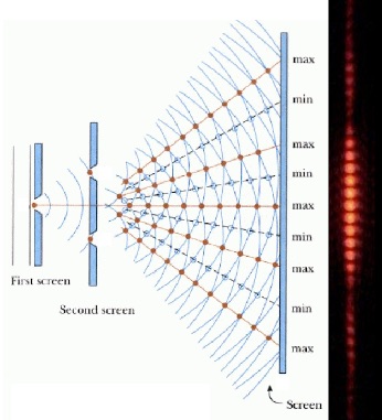
The infamous Double Slit experiment demonstrates a single photon going through two (or more) slits simultaneously. The “beats” of light are caused by photons interfering like waves between the two slits. This still works if you release one photon at a time; even individually, they’ll only hit the bright regions.
Instead of the photons going straight through and creating a single bright spot behind every slit (classical) we instead see a wave interference pattern (quantum). This only makes sense if: 1) the photons of light act like waves and 2) they’re going through both slits.
It’s completely natural to suspect that the objects involved in experiments like this are really in only one state, but have behaviors too complex for us to understand. Rather surprisingly, we can pretty effectively rule that out.
There is no scale at which quantum effects stop working
To date, every experiment capable of detecting the difference between quantum and classical results has always demonstrated that the underlying behavior is strictly quantum. To be fair, quantum phenomena is as delicate as delicate can be. For example, in the double slit experiment any interaction that could indicate to the outside world (the “environment”), even in principle, which slit the particle went through will destroy the quantumness of the experiment (the interference fringes go away). When you have to worry about the disruptive influence of individual stray particles, you don’t expect to see quantum effects on the scale of people and planets.
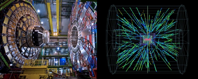
That said, the double slit experiment has been done and works for every kind of particle and even molecules with hundreds of atoms. Quantum states can be maintained for minutes or hours, so superposition doesn’t “wear out” on its own. Needles large enough to be seen with the naked eye have been put into superpositions of vibrational modes and this year China launched the first quantum communication satellite which is being used as a relay to establish quantum effects over scales of hundreds or thousands of miles. So far there is no indication of a natural scale where objects are big enough, far enough apart, or old enough that quantum mechanics simply cease to apply. The only limits seem to be in our engineering abilities. It’s completely infeasible to do experimental quantum physics with something as substantive as a person (or really anything close).
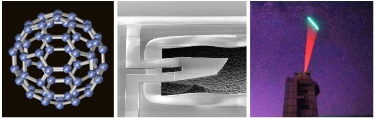
Left: Buckminsterfullerene (and even much larger molecules) interfere in double-slit experiments. Middle: A needle that was put into a superposition of literally both vibrating and not vibrating at all. Right: Time lapse of a laser being used to establish quantum entanglement with carefully isolated atoms inside of a satellite in orbit.
If the quantum laws did simply ceased to apply at some scale, then those laws would be bizarre and unique; the first of their kind. Every physical law applies at all scales, it’s just a question of how relevant each is. For example, on large scales gravity is practically the only force worth worrying about, but on the atomic scale it can be efficiently ignored (usually).

Io sticks to (orbits) Jupiter because of gravitational forces and styrofoam sticks to cats because of electrical forces. Both apply on all scales, but on smaller scales (evidently cat scale and below) electrical forces tend to dominate.
So here comes the point: if the quantum laws really do apply at all scales, then we should expect that exactly like everything else, people (no big deal) should ultimately follow quantum laws and exhibit quantum behavior. Including superposition. But that begs a very natural question: what does it feel like to be in multiple states? Why don’t we notice?
The quantum laws don’t contradict the world we see
When you first hear about the heliocentric theory (the Earth is in motion around the Sun instead of the other way around), the first question that naturally comes to mind is “Why don’t I feel the Earth moving?“. But in trying to answer that you find yourself trying to climb out of the assumption that you should notice anything. A more enlightening question is “What do the laws of gravitation and motion say that we should experience?“. In the case of Newton’s laws and the Earth, we find that because the surface of the Earth, the air above it, and the people on it all travel together, we shouldn’t feel anything. Despite moving at ridiculous speeds there are only subtle tell-tail signs that we’re moving at all, like ocean tides or the precession of garishly large pendulums.
Quantum laws are in a similar situation. You may have noticed that you’ve never met other versions of yourself wandering around your house. You’re there, so shouldn’t at least some other versions of you be as well? Why don’t we see them? A better question is “What do the quantum laws say that we should experience?“.

Why don’t we run into our other versions all the time, instead of absolutely never?
The Correspondence Principle is arguably one of the most important philosophical underpinnings in science. It says that whatever your theories are, they need to predict (or at the very least not contradict) ordinary physical laws and ordinary experience when applied to ordinary situations.
When you apply the laws of relativity to speeds much slower than light all of the length contractions and twin paradoxes become less and less important until the laws we’re accustomed to working with are more than sufficient. That is to say; while we can detect relativistic effects all the way down to walking speed, the effect is so small that you don’t need to worry about it when you’re walking.
Similarly, the quantum laws reproduce the classical laws when you assume that there are far more particles around than you can keep track of and that they’re not particularly correlated with one another (i.e., if you’re watching one air molecule there’s really no telling what the next will be doing). There are times when this assumption doesn’t hold, but those are exactly the cases that reveal that the quantum laws are there.
It turns out that simply applying the quantum laws to everything seems to resolve all the big paradoxes. That’s good on the one hand because physics works. But on the other hand, we’re forced into the suspicion that the our universe might be needlessly weird.
The big rift between “the quantum world” and “the classical world” is that large things, like you and literally everything that you can see, always seem to be in exactly one state. When we keep quantum systems carefully isolated (usually by making them very cold, very tiny, and very dark) we find that they exhibit superposition, but when we then interact with those quantum systems they “decohere” and are found to be in a smaller set of states. This is sometimes called “wave function collapse”, to evoke an image of a wide wave suddenly collapsing into a single tiny particle. The rule seems to be that interacting with things makes their behavior more classical.
But not always. “Wave function collapse” doesn’t happen when isolated quantum systems interact with each other, only when they interact with the environment (the outside world). Experimentally, when you allow a couple of systems that are both in a superposition of states to interact, then the result is two systems in a joint superposition of states (this is entanglement). If the rule were as simple as “when things interact they decohere” you’d expect to find both systems each in only one state after interacting. What we find instead is that in every testable case the superposition in maintained. Changed or entangled, sure, but the various states in a superposition never just disappear. When you interact with a system in a superposition you only see a particular state, not a superposition. So what’s going on when we, or anything in the environment, interacts with a quantum system? Where did the other states in the superposition go?
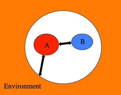
We have physical laws that describe the interactions between pairs of isolated quantum systems (A and B). When we treat the environment as another (albeit very big) quantum system we can continue to use those same laws. When we assume that the environment is not a quantum system, we have to make up new laws and special exceptions.
The rules we use to describe how pairs of isolated systems interact also do an excellent job describing the way isolated quantum systems interact with the outside environment. When isolated systems interact with each other they become entangled. When isolated systems interact with the environment they decohere. It turns out that these two effects, entanglement and decoherence, are two sides of the same coin. When we make the somewhat artificial choice to ask “What states of system B can some particular state in system A interact with?” we find that the result mirrors what we ourselves see when we interact with things and “collapse their wave functions” (see the Answer Gravy below for more on that). The phrase “wave function collapse” is like the word “sunrise”; it does a good job describing our personal experience, but does a terrible job describing the underlying dynamics. When you ask the natural question “What does it feel like to be in a many different states?” the frustrating answer seems to be “You tell me.“.
A thing can only be inferred to be in multiple states (such as by witnessing an interference pattern). If there’s any way to tell the difference between the individual states that make up a superposition, then (from your point of view) there is no superposition. Since you can see yourself, you can tell the difference between your state and another. You might be in an effectively infinite number of states, but you’d never know it. The fact that you can’t help but observe yourself means that you will never observe yourself somewhere that you’re not.
“Where are my other versions?” isn’t quite the right question
Where are those other versions of you? Assuming that they exist, they’re no place more mysterious than where you are now. In the double slit experiment different versions of the same object go through the different slits and you can literally point to exactly where each version is (in exactly the same way you can point at anything you can’t presently observe), so the physical position of each version isn’t a mystery.
The mathematical operations that describe quantum mechanical interactions and the passage of time are “linear”, which means that they treat the different states in a superposition separately. A linear operator does the same thing to every state individually, and then sums the results. There are a lot of examples of linear phenomena in nature, including waves (which are solutions to the wave equation). The Schrodinger equation, which describe how quantum wave functions behave, is also linear.

The wave equation is linear, so you can describe how each of these ways travels across the surface of the water by considering them each one at a time and adding up the results. They don’t interact with each other directly, but they do add up.
So, if there are other versions of you, they’re wandering around in very much the same way you are. But (as you may have noticed) you don’t interact with them, so saying they’re “in the same place you are” isn’t particularly useful. Which is frustrating in a chained-in-Plato’s-cave-kind-of-way.
The rain puddle picture is from here.
Answer Gravy: In quantum mechanics the affect of the passage of time and every interaction is described by a linear operator (even better, it’s a unitary operator). Linear operators treat everything they’re given separately, as though each piece was the only piece. In mathspeak, if ") is a linear operator, then
is a linear operator, then  = af(x)+bf(y)") (where
(where  and
and  are ordinary numbers). The output is a sum of the results from every input taken individually.
Consider a quantum system that can be in either of two states,  or
or  . When observed it is always found to be in only one of the states, but when left in isolation it can be in any superposition of the form
  , where
  . The
. The  and
and  are important for how this state will interact with others as well as describing the probability of seeing either result. According to the Born Rule, if
  (for example), then the probability of seeing is
  .
.
Let’s also say that the quantum scientists Alice and Bob can be described by the modest notation \rangle") and
and \rangle") , where the “?” indicates that they have not looked at the isolated quantum system yet. If the isolated system is in the state initially, then the initial state of the whole scenario is
, where the “?” indicates that they have not looked at the isolated quantum system yet. If the isolated system is in the state initially, then the initial state of the whole scenario is \rangle|B(?)\rangle|\blacksquare\rangle") .
.
Define a linear “look” operation for Alice,  , that works like this
\rangle|B(?)\rangle|\blacksquare\rangle\right) = |A(\blacksquare)\rangle|B(?)\rangle|\blacksquare\rangle")
and similarly for Bob
\rangle|B(?)\rangle|\blacksquare\rangle\right) = |A(?)\rangle|B(\blacksquare)\rangle|\blacksquare\rangle")
Applying these one at a time we see what happens when each looks at the quantum system; they end up seeing the same thing.
\rangle|B(?)\rangle|\blacksquare\rangle\right) = L_B\left(|A(\blacksquare)\rangle|B(?)\rangle|\blacksquare\rangle\right) = |A(\blacksquare)\rangle|B(\blacksquare)\rangle|\blacksquare\rangle")
It’s subtle, but you’ll notice that the coefficient in front of this state is 1, meaning that it has a 100% of happening.
But what happens if the system is in a superposition of states, such as  ? Since the “look” operation is linear, this is no big deal.
![\begin{array}{ll} &L_BL_A\left(|A(?)\rangle|B(?)\rangle\left(\frac{|\square\rangle+|\blacksquare\rangle}{\sqrt{2}}\right)\right) \\[2mm] =&\frac{1}{\sqrt{2}}L_BL_A\left(|A(?)\rangle|B(?)\rangle|\square\rangle\right)+\frac{1}{\sqrt{2}}L_BL_A\left(|A(?)\rangle|B(?)\rangle|\blacksquare\rangle\right) \\[2mm] =&\frac{1}{\sqrt{2}}L_B\left(|A(\square)\rangle|B(?)\rangle|\square\rangle\right)+\frac{1}{\sqrt{2}}L_B\left(|A(\blacksquare)\rangle|B(?)\rangle|\blacksquare\rangle\right) \\[2mm] =&\frac{1}{\sqrt{2}}|A(\square)\rangle|B(\square)\rangle|\square\rangle+\frac{1}{\sqrt{2}}|A(\blacksquare)\rangle|B(\blacksquare)\rangle|\blacksquare\rangle \\[2mm] \end{array}](//s0.wp.com/latex.php?latex=%5Cbegin%7Barray%7D%7Bll%7D+%26L_BL_A%5Cleft%28%7CA%28%3F%29%5Crangle%7CB%28%3F%29%5Crangle%5Cleft%28%5Cfrac%7B%7C%5Csquare%5Crangle%2B%7C%5Cblacksquare%5Crangle%7D%7B%5Csqrt%7B2%7D%7D%5Cright%29%5Cright%29+%5C%5C%5B2mm%5D+%3D%26%5Cfrac%7B1%7D%7B%5Csqrt%7B2%7D%7DL_BL_A%5Cleft%28%7CA%28%3F%29%5Crangle%7CB%28%3F%29%5Crangle%7C%5Csquare%5Crangle%5Cright%29%2B%5Cfrac%7B1%7D%7B%5Csqrt%7B2%7D%7DL_BL_A%5Cleft%28%7CA%28%3F%29%5Crangle%7CB%28%3F%29%5Crangle%7C%5Cblacksquare%5Crangle%5Cright%29+%5C%5C%5B2mm%5D+%3D%26%5Cfrac%7B1%7D%7B%5Csqrt%7B2%7D%7DL_B%5Cleft%28%7CA%28%5Csquare%29%5Crangle%7CB%28%3F%29%5Crangle%7C%5Csquare%5Crangle%5Cright%29%2B%5Cfrac%7B1%7D%7B%5Csqrt%7B2%7D%7DL_B%5Cleft%28%7CA%28%5Cblacksquare%29%5Crangle%7CB%28%3F%29%5Crangle%7C%5Cblacksquare%5Crangle%5Cright%29+%5C%5C%5B2mm%5D+%3D%26%5Cfrac%7B1%7D%7B%5Csqrt%7B2%7D%7D%7CA%28%5Csquare%29%5Crangle%7CB%28%5Csquare%29%5Crangle%7C%5Csquare%5Crangle%2B%5Cfrac%7B1%7D%7B%5Csqrt%7B2%7D%7D%7CA%28%5Cblacksquare%29%5Crangle%7CB%28%5Cblacksquare%29%5Crangle%7C%5Cblacksquare%5Crangle+%5C%5C%5B2mm%5D+%5Cend%7Barray%7D&bg=ffffff&fg=000&s=0 "\begin{array}{ll} &L_BL_A\left(|A(?)\rangle|B(?)\rangle\left(\frac{|\square\rangle+|\blacksquare\rangle}{\sqrt{2}}\right)\right) \\[2mm] =&\frac{1}{\sqrt{2}}L_BL_A\left(|A(?)\rangle|B(?)\rangle|\square\rangle\right)+\frac{1}{\sqrt{2}}L_BL_A\left(|A(?)\rangle|B(?)\rangle|\blacksquare\rangle\right) \\[2mm] =&\frac{1}{\sqrt{2}}L_B\left(|A(\square)\rangle|B(?)\rangle|\square\rangle\right)+\frac{1}{\sqrt{2}}L_B\left(|A(\blacksquare)\rangle|B(?)\rangle|\blacksquare\rangle\right) \\[2mm] =&\frac{1}{\sqrt{2}}|A(\square)\rangle|B(\square)\rangle|\square\rangle+\frac{1}{\sqrt{2}}|A(\blacksquare)\rangle|B(\blacksquare)\rangle|\blacksquare\rangle \\[2mm] \end{array}")
From an extremely outside perspective, Alice and Bob have a probability of  of seeing either state. Alice, Bob, and their pet quantum system are all in a joint superposition of states: they’re entangled.
Anything else that happens can also be described by a linear operation (call it “F”) and therefore these two states can’t directly affect each other.
\rangle|B(\square)\rangle|\square\rangle+\frac{1}{\sqrt{2}}|A(\blacksquare)\rangle|B(\blacksquare)\rangle|\blacksquare\rangle\right) = \frac{1}{\sqrt{2}}F\left(|A(\square)\rangle|B(\square)\rangle|\square\rangle\right)+\frac{1}{\sqrt{2}}F\left(|A(\blacksquare)\rangle|B(\blacksquare)\rangle|\blacksquare\rangle\right)")
The states can both contribute to the same end result, but only for other systems/observers that haven’t interacted with either of Alice or Bob or their pet quantum system. We see this in the double slit experiment: the versions of the photons that go through each slit each contribute to the interference pattern on the screen, but neither version ever directly affects the other. “Contributing but not interacting” sounds more abstract than it is. If you shine two lights on the same object, the photons flying around all ignore each other, but each individually contributes to illuminating said object just fine.
The Alices and Bobs in the states \rangle|B(\square)\rangle|\square\rangle") and
and \rangle|B(\blacksquare)\rangle|\blacksquare\rangle") consider themselves to be the only ones (they don’t interact with their other versions). The version of Alice in the state
consider themselves to be the only ones (they don’t interact with their other versions). The version of Alice in the state \rangle") “feels” that the state of the universe is because, as long as the operators being applied are linear, it doesn’t matter in any way if the other state exists.
“feels” that the state of the universe is because, as long as the operators being applied are linear, it doesn’t matter in any way if the other state exists.
Notice that Alice and Bob don’t see their own state being modified by that  . They don’t see their state as being 50% likely, they see it as definitely happening (every version thinks that). That can be fixed with a “normalizing constant“. That sounds more exciting than it is. If you ask “what is the probability of rolling a 4 on a die?” the answer is “1/6”. If you are then told that the number rolled was even, then suddenly the probability jumps to 1/3. Once 1, 3, and 5 are ruled out, while the probability of 2, 4, and 6 change from 1/6 each to 1/3 each. Same idea here; every version of Alice and Bob is certain of their result, and multiplying their state by the normalizing constant (
 in this example) reflects that sentiment and ensures that probabilities sum to 1.
If you are determined to follow a particular state through the problem, ignoring the others, then you need to make this adjustment. The interaction operation starts to look more like a “projection operator” adjusted so that the resulting state is properly normalized.
The projection operator for the state is  . This Bra-Ket notation allows us to quickly write vectors, , and their duals,
  , and their inner products,
  . This particular inner product, , is the probability of measuring when looking at the state . This can be tricky, but in this example we’re assuming “orthogonal states”. In mathspeak,
  and
and  .
.
An interaction with the system in the state  performs the operation
  with probability
  or
or  with probability
  .
.
Here comes the same example again, but in a more “wave function collapse sort of way”. We still start with the state \rangle|B(?)\rangle\left(\frac{|\square\rangle+|\blacksquare\rangle}{\sqrt{2}}\right)") , but when Alice or Bob looks at the system (or perhaps a little before or a little after) the wave function of the state collapses. It needs to be one or the other, so the quantum system suddenly and inexplicably becomes
, but when Alice or Bob looks at the system (or perhaps a little before or a little after) the wave function of the state collapses. It needs to be one or the other, so the quantum system suddenly and inexplicably becomes
![\begin{array}{ll} &M_\blacksquare\left(\frac{|\square\rangle+|\blacksquare\rangle}{\sqrt{2}}\right) \\[2mm] =& \frac{|\blacksquare\rangle\langle\blacksquare|\left(\frac{|\square\rangle+|\blacksquare\rangle}{\sqrt{2}}\right)}{\left|\langle\blacksquare|\left(\frac{|\square\rangle+|\blacksquare\rangle}{\sqrt{2}}\right)\right|} \\[2mm] =& \frac{|\blacksquare\rangle\left(\frac{\langle\blacksquare|\square\rangle+\langle\blacksquare|\blacksquare\rangle}{\sqrt{2}}\right)}{\left|\frac{\langle\blacksquare|\square\rangle+\langle\blacksquare|\blacksquare\rangle}{\sqrt{2}}\right|} \\[2mm] =& \frac{|\blacksquare\rangle\left(\frac{0+1}{\sqrt{2}}\right)}{\left|\frac{0+1}{\sqrt{2}}\right|} \\[2mm] =& \frac{|\blacksquare\rangle\frac{1}{\sqrt{2}}}{\frac{1}{\sqrt{2}}} \\[2mm] =& |\blacksquare\rangle \end{array}](//s0.wp.com/latex.php?latex=%5Cbegin%7Barray%7D%7Bll%7D+%26M_%5Cblacksquare%5Cleft%28%5Cfrac%7B%7C%5Csquare%5Crangle%2B%7C%5Cblacksquare%5Crangle%7D%7B%5Csqrt%7B2%7D%7D%5Cright%29+%5C%5C%5B2mm%5D+%3D%26+%5Cfrac%7B%7C%5Cblacksquare%5Crangle%5Clangle%5Cblacksquare%7C%5Cleft%28%5Cfrac%7B%7C%5Csquare%5Crangle%2B%7C%5Cblacksquare%5Crangle%7D%7B%5Csqrt%7B2%7D%7D%5Cright%29%7D%7B%5Cleft%7C%5Clangle%5Cblacksquare%7C%5Cleft%28%5Cfrac%7B%7C%5Csquare%5Crangle%2B%7C%5Cblacksquare%5Crangle%7D%7B%5Csqrt%7B2%7D%7D%5Cright%29%5Cright%7C%7D+%5C%5C%5B2mm%5D+%3D%26+%5Cfrac%7B%7C%5Cblacksquare%5Crangle%5Cleft%28%5Cfrac%7B%5Clangle%5Cblacksquare%7C%5Csquare%5Crangle%2B%5Clangle%5Cblacksquare%7C%5Cblacksquare%5Crangle%7D%7B%5Csqrt%7B2%7D%7D%5Cright%29%7D%7B%5Cleft%7C%5Cfrac%7B%5Clangle%5Cblacksquare%7C%5Csquare%5Crangle%2B%5Clangle%5Cblacksquare%7C%5Cblacksquare%5Crangle%7D%7B%5Csqrt%7B2%7D%7D%5Cright%7C%7D+%5C%5C%5B2mm%5D+%3D%26+%5Cfrac%7B%7C%5Cblacksquare%5Crangle%5Cleft%28%5Cfrac%7B0%2B1%7D%7B%5Csqrt%7B2%7D%7D%5Cright%29%7D%7B%5Cleft%7C%5Cfrac%7B0%2B1%7D%7B%5Csqrt%7B2%7D%7D%5Cright%7C%7D+%5C%5C%5B2mm%5D+%3D%26+%5Cfrac%7B%7C%5Cblacksquare%5Crangle%5Cfrac%7B1%7D%7B%5Csqrt%7B2%7D%7D%7D%7B%5Cfrac%7B1%7D%7B%5Csqrt%7B2%7D%7D%7D+%5C%5C%5B2mm%5D+%3D%26+%7C%5Cblacksquare%5Crangle+%5Cend%7Barray%7D&bg=ffffff&fg=000&s=0 "\begin{array}{ll} &M_\blacksquare\left(\frac{|\square\rangle+|\blacksquare\rangle}{\sqrt{2}}\right) \\[2mm] =& \frac{|\blacksquare\rangle\langle\blacksquare|\left(\frac{|\square\rangle+|\blacksquare\rangle}{\sqrt{2}}\right)}{\left|\langle\blacksquare|\left(\frac{|\square\rangle+|\blacksquare\rangle}{\sqrt{2}}\right)\right|} \\[2mm] =& \frac{|\blacksquare\rangle\left(\frac{\langle\blacksquare|\square\rangle+\langle\blacksquare|\blacksquare\rangle}{\sqrt{2}}\right)}{\left|\frac{\langle\blacksquare|\square\rangle+\langle\blacksquare|\blacksquare\rangle}{\sqrt{2}}\right|} \\[2mm] =& \frac{|\blacksquare\rangle\left(\frac{0+1}{\sqrt{2}}\right)}{\left|\frac{0+1}{\sqrt{2}}\right|} \\[2mm] =& \frac{|\blacksquare\rangle\frac{1}{\sqrt{2}}}{\frac{1}{\sqrt{2}}} \\[2mm] =& |\blacksquare\rangle \end{array}")
That is to say, the superposition suddenly becomes only the measured state while the other states suddenly vanish (by some totally unknown means). After this collapse, the “look” operators function normally.
This “measurement operator” (which does all the collapsing) is definitively non-linear, which is a big red flag. We never see non-linear operations when we study isolated sets of quantum systems, no matter how they interact. The one and only time we see non-linear operations is when we include the environment and even then only when we assume that there’s something unique and special about the environment. When you assume that literally everything is a quantum system capable of being in superpositions of states the quantum laws become ontologically parsimonious (easy to write down). We lose our special position as the only version of us that exists, but we gain a system of physical laws that doesn’t involve lots of weird exceptions, extra rules, and paradoxes.
=115")
=100(1+0.15)^2=132.25")
=100(1+0.15)^3=152.09")
^N")

![\begin{array}{ll} &L_BL_A\left(|A(?)\rangle|B(?)\rangle\left(\frac{|\square\rangle+|\blacksquare\rangle}{\sqrt{2}}\right)\right) \\[2mm] =&\frac{1}{\sqrt{2}}L_BL_A\left(|A(?)\rangle|B(?)\rangle|\square\rangle\right)+\frac{1}{\sqrt{2}}L_BL_A\left(|A(?)\rangle|B(?)\rangle|\blacksquare\rangle\right) \\[2mm] =&\frac{1}{\sqrt{2}}L_B\left(|A(\square)\rangle|B(?)\rangle|\square\rangle\right)+\frac{1}{\sqrt{2}}L_B\left(|A(\blacksquare)\rangle|B(?)\rangle|\blacksquare\rangle\right) \\[2mm] =&\frac{1}{\sqrt{2}}|A(\square)\rangle|B(\square)\rangle|\square\rangle+\frac{1}{\sqrt{2}}|A(\blacksquare)\rangle|B(\blacksquare)\rangle|\blacksquare\rangle \\[2mm] \end{array}](http://s0.wp.com/latex.php?latex=%5Cbegin%7Barray%7D%7Bll%7D+%26L_BL_A%5Cleft%28%7CA%28%3F%29%5Crangle%7CB%28%3F%29%5Crangle%5Cleft%28%5Cfrac%7B%7C%5Csquare%5Crangle%2B%7C%5Cblacksquare%5Crangle%7D%7B%5Csqrt%7B2%7D%7D%5Cright%29%5Cright%29+%5C%5C%5B2mm%5D+%3D%26%5Cfrac%7B1%7D%7B%5Csqrt%7B2%7D%7DL_BL_A%5Cleft%28%7CA%28%3F%29%5Crangle%7CB%28%3F%29%5Crangle%7C%5Csquare%5Crangle%5Cright%29%2B%5Cfrac%7B1%7D%7B%5Csqrt%7B2%7D%7DL_BL_A%5Cleft%28%7CA%28%3F%29%5Crangle%7CB%28%3F%29%5Crangle%7C%5Cblacksquare%5Crangle%5Cright%29+%5C%5C%5B2mm%5D+%3D%26%5Cfrac%7B1%7D%7B%5Csqrt%7B2%7D%7DL_B%5Cleft%28%7CA%28%5Csquare%29%5Crangle%7CB%28%3F%29%5Crangle%7C%5Csquare%5Crangle%5Cright%29%2B%5Cfrac%7B1%7D%7B%5Csqrt%7B2%7D%7DL_B%5Cleft%28%7CA%28%5Cblacksquare%29%5Crangle%7CB%28%3F%29%5Crangle%7C%5Cblacksquare%5Crangle%5Cright%29+%5C%5C%5B2mm%5D+%3D%26%5Cfrac%7B1%7D%7B%5Csqrt%7B2%7D%7D%7CA%28%5Csquare%29%5Crangle%7CB%28%5Csquare%29%5Crangle%7C%5Csquare%5Crangle%2B%5Cfrac%7B1%7D%7B%5Csqrt%7B2%7D%7D%7CA%28%5Cblacksquare%29%5Crangle%7CB%28%5Cblacksquare%29%5Crangle%7C%5Cblacksquare%5Crangle+%5C%5C%5B2mm%5D+%5Cend%7Barray%7D&bg=ffffff&fg=000&s=0 "\begin{array}{ll} &L_BL_A\left(|A(?)\rangle|B(?)\rangle\left(\frac{|\square\rangle+|\blacksquare\rangle}{\sqrt{2}}\right)\right) \\[2mm] =&\frac{1}{\sqrt{2}}L_BL_A\left(|A(?)\rangle|B(?)\rangle|\square\rangle\right)+\frac{1}{\sqrt{2}}L_BL_A\left(|A(?)\rangle|B(?)\rangle|\blacksquare\rangle\right) \\[2mm] =&\frac{1}{\sqrt{2}}L_B\left(|A(\square)\rangle|B(?)\rangle|\square\rangle\right)+\frac{1}{\sqrt{2}}L_B\left(|A(\blacksquare)\rangle|B(?)\rangle|\blacksquare\rangle\right) \\[2mm] =&\frac{1}{\sqrt{2}}|A(\square)\rangle|B(\square)\rangle|\square\rangle+\frac{1}{\sqrt{2}}|A(\blacksquare)\rangle|B(\blacksquare)\rangle|\blacksquare\rangle \\[2mm] \end{array}")
![\begin{array}{ll} &M_\blacksquare\left(\frac{|\square\rangle+|\blacksquare\rangle}{\sqrt{2}}\right) \\[2mm] =& \frac{|\blacksquare\rangle\langle\blacksquare|\left(\frac{|\square\rangle+|\blacksquare\rangle}{\sqrt{2}}\right)}{\left|\langle\blacksquare|\left(\frac{|\square\rangle+|\blacksquare\rangle}{\sqrt{2}}\right)\right|} \\[2mm] =& \frac{|\blacksquare\rangle\left(\frac{\langle\blacksquare|\square\rangle+\langle\blacksquare|\blacksquare\rangle}{\sqrt{2}}\right)}{\left|\frac{\langle\blacksquare|\square\rangle+\langle\blacksquare|\blacksquare\rangle}{\sqrt{2}}\right|} \\[2mm] =& \frac{|\blacksquare\rangle\left(\frac{0+1}{\sqrt{2}}\right)}{\left|\frac{0+1}{\sqrt{2}}\right|} \\[2mm] =& \frac{|\blacksquare\rangle\frac{1}{\sqrt{2}}}{\frac{1}{\sqrt{2}}} \\[2mm] =& |\blacksquare\rangle \end{array}](http://s0.wp.com/latex.php?latex=%5Cbegin%7Barray%7D%7Bll%7D+%26M_%5Cblacksquare%5Cleft%28%5Cfrac%7B%7C%5Csquare%5Crangle%2B%7C%5Cblacksquare%5Crangle%7D%7B%5Csqrt%7B2%7D%7D%5Cright%29+%5C%5C%5B2mm%5D+%3D%26+%5Cfrac%7B%7C%5Cblacksquare%5Crangle%5Clangle%5Cblacksquare%7C%5Cleft%28%5Cfrac%7B%7C%5Csquare%5Crangle%2B%7C%5Cblacksquare%5Crangle%7D%7B%5Csqrt%7B2%7D%7D%5Cright%29%7D%7B%5Cleft%7C%5Clangle%5Cblacksquare%7C%5Cleft%28%5Cfrac%7B%7C%5Csquare%5Crangle%2B%7C%5Cblacksquare%5Crangle%7D%7B%5Csqrt%7B2%7D%7D%5Cright%29%5Cright%7C%7D+%5C%5C%5B2mm%5D+%3D%26+%5Cfrac%7B%7C%5Cblacksquare%5Crangle%5Cleft%28%5Cfrac%7B%5Clangle%5Cblacksquare%7C%5Csquare%5Crangle%2B%5Clangle%5Cblacksquare%7C%5Cblacksquare%5Crangle%7D%7B%5Csqrt%7B2%7D%7D%5Cright%29%7D%7B%5Cleft%7C%5Cfrac%7B%5Clangle%5Cblacksquare%7C%5Csquare%5Crangle%2B%5Clangle%5Cblacksquare%7C%5Cblacksquare%5Crangle%7D%7B%5Csqrt%7B2%7D%7D%5Cright%7C%7D+%5C%5C%5B2mm%5D+%3D%26+%5Cfrac%7B%7C%5Cblacksquare%5Crangle%5Cleft%28%5Cfrac%7B0%2B1%7D%7B%5Csqrt%7B2%7D%7D%5Cright%29%7D%7B%5Cleft%7C%5Cfrac%7B0%2B1%7D%7B%5Csqrt%7B2%7D%7D%5Cright%7C%7D+%5C%5C%5B2mm%5D+%3D%26+%5Cfrac%7B%7C%5Cblacksquare%5Crangle%5Cfrac%7B1%7D%7B%5Csqrt%7B2%7D%7D%7D%7B%5Cfrac%7B1%7D%7B%5Csqrt%7B2%7D%7D%7D+%5C%5C%5B2mm%5D+%3D%26+%7C%5Cblacksquare%5Crangle+%5Cend%7Barray%7D&bg=ffffff&fg=000&s=0 "\begin{array}{ll} &M_\blacksquare\left(\frac{|\square\rangle+|\blacksquare\rangle}{\sqrt{2}}\right) \\[2mm] =& \frac{|\blacksquare\rangle\langle\blacksquare|\left(\frac{|\square\rangle+|\blacksquare\rangle}{\sqrt{2}}\right)}{\left|\langle\blacksquare|\left(\frac{|\square\rangle+|\blacksquare\rangle}{\sqrt{2}}\right)\right|} \\[2mm] =& \frac{|\blacksquare\rangle\left(\frac{\langle\blacksquare|\square\rangle+\langle\blacksquare|\blacksquare\rangle}{\sqrt{2}}\right)}{\left|\frac{\langle\blacksquare|\square\rangle+\langle\blacksquare|\blacksquare\rangle}{\sqrt{2}}\right|} \\[2mm] =& \frac{|\blacksquare\rangle\left(\frac{0+1}{\sqrt{2}}\right)}{\left|\frac{0+1}{\sqrt{2}}\right|} \\[2mm] =& \frac{|\blacksquare\rangle\frac{1}{\sqrt{2}}}{\frac{1}{\sqrt{2}}} \\[2mm] =& |\blacksquare\rangle \end{array}")
 . What this means is that no matter how close you want to get to 1, you can get closer than that with enough 9’s. If the 9’s never end, then the difference between 1 and 0.999… is zero.

(B-1)(B-1)\ldots_B") . Showing that this is equal to one is a matter of working this around until it looks like a geometric sum,
. Showing that this is equal to one is a matter of working this around until it looks like a geometric sum,  , and using the fact that
  .
.![\begin{array}{ll} &0.(B-1)(B-1)(B-1)\ldots_B \\[2mm] =& (B-1)\times B^{-1}+(B-1)\times B^{-1}+(B-1)\times B^{-1}+\ldots \\[2mm] =& \sum_{n=1}^\infty (B-1)\times B^{-n} \\[2mm] =& \sum_{n=0}^\infty (B-1)\times B^{-n-1} \\[2mm] =& \sum_{n=0}^\infty \frac{B-1}{B}\times B^{-n} \\[2mm] =& \frac{B-1}{B}\sum_{n=0}^\infty B^{-n} \\[2mm] =& \frac{B-1}{B}\sum_{n=0}^\infty \left(\frac{1}{B}\right)^n \\[2mm] =& \frac{B-1}{B} \frac{1}{1-\frac{1}{B}} \\[2mm] =& \frac{B-1}{B} \frac{B}{B-1} \\[2mm] =& \frac{B-1}{B} \frac{B}{B-1} \\[2mm] =&1 \end{array}](http://s0.wp.com/latex.php?latex=%5Cbegin%7Barray%7D%7Bll%7D++%260.%28B-1%29%28B-1%29%28B-1%29%5Cldots_B+%5C%5C%5B2mm%5D++%3D%26+%28B-1%29%5Ctimes+B%5E%7B-1%7D%2B%28B-1%29%5Ctimes+B%5E%7B-1%7D%2B%28B-1%29%5Ctimes+B%5E%7B-1%7D%2B%5Cldots+%5C%5C%5B2mm%5D++%3D%26+%5Csum_%7Bn%3D1%7D%5E%5Cinfty+%28B-1%29%5Ctimes+B%5E%7B-n%7D+%5C%5C%5B2mm%5D++%3D%26+%5Csum_%7Bn%3D0%7D%5E%5Cinfty+%28B-1%29%5Ctimes+B%5E%7B-n-1%7D+%5C%5C%5B2mm%5D++%3D%26+%5Csum_%7Bn%3D0%7D%5E%5Cinfty+%5Cfrac%7BB-1%7D%7BB%7D%5Ctimes+B%5E%7B-n%7D+%5C%5C%5B2mm%5D++%3D%26+%5Cfrac%7BB-1%7D%7BB%7D%5Csum_%7Bn%3D0%7D%5E%5Cinfty+B%5E%7B-n%7D+%5C%5C%5B2mm%5D++%3D%26+%5Cfrac%7BB-1%7D%7BB%7D%5Csum_%7Bn%3D0%7D%5E%5Cinfty+%5Cleft%28%5Cfrac%7B1%7D%7BB%7D%5Cright%29%5En+%5C%5C%5B2mm%5D++%3D%26+%5Cfrac%7BB-1%7D%7BB%7D+%5Cfrac%7B1%7D%7B1-%5Cfrac%7B1%7D%7BB%7D%7D+%5C%5C%5B2mm%5D++%3D%26+%5Cfrac%7BB-1%7D%7BB%7D+%5Cfrac%7BB%7D%7BB-1%7D+%5C%5C%5B2mm%5D++%3D%26+%5Cfrac%7BB-1%7D%7BB%7D+%5Cfrac%7BB%7D%7BB-1%7D+%5C%5C%5B2mm%5D++%3D%261++%5Cend%7Barray%7D&bg=ffffff&fg=000&s=0 "\begin{array}{ll} &0.(B-1)(B-1)(B-1)\ldots_B \\[2mm] =& (B-1)\times B^{-1}+(B-1)\times B^{-1}+(B-1)\times B^{-1}+\ldots \\[2mm] =& \sum_{n=1}^\infty (B-1)\times B^{-n} \\[2mm] =& \sum_{n=0}^\infty (B-1)\times B^{-n-1} \\[2mm] =& \sum_{n=0}^\infty \frac{B-1}{B}\times B^{-n} \\[2mm] =& \frac{B-1}{B}\sum_{n=0}^\infty B^{-n} \\[2mm] =& \frac{B-1}{B}\sum_{n=0}^\infty \left(\frac{1}{B}\right)^n \\[2mm] =& \frac{B-1}{B} \frac{1}{1-\frac{1}{B}} \\[2mm] =& \frac{B-1}{B} \frac{B}{B-1} \\[2mm] =& \frac{B-1}{B} \frac{B}{B-1} \\[2mm] =&1 \end{array}")
 when B=1. So don’t use base 1. There are

 . This equation isn’t exact, but (for N bigger than ten or so) it’s way too close to matter.
 and about 10% for
  . This gives us a decent rule of thumb: in practice, if you’re drawing objects at random and you haven’t seen any repeats in the first K draws, then there are likely to be at least
  objects in the set. Or, to be
  times without repeats.

 , which is both admittedly weird looking and remarkably accurate. This can be solved for K.
 - N\ln\left(\ln\left(\frac{1}{P}\right)\right)")
\right)") is between -1 and 1. You’re likely to finally see every object at least once somewhere in
is between -1 and 1. You’re likely to finally see every object at least once somewhere in \ln(N)<K<(N+1)\ln(N)") . You’ll already know approximately how many objects there are (N), because you’ve already seen (almost) all of them.
. You’ll already know approximately how many objects there are (N), because you’ve already seen (almost) all of them.
") times, then you’ve probably seen everything. Or in slightly more back-of-the-envelope-useful terms: when you’ve drawn more than “K = 2N times the number of digits in K” times.
times, then you’ve probably seen everything. Or in slightly more back-of-the-envelope-useful terms: when you’ve drawn more than “K = 2N times the number of digits in K” times. ) and subtract all of the sequences that are missing one of the letters. The number of sequences missing a particular letter is
 ^K") and there are N letters, so the total number of sequences missing at least one letter is
and there are N letters, so the total number of sequences missing at least one letter is ^K") . But if you remove all the sequences without an A and all the sequences without a B, then you’ve twice removed all the sequences missing both A’s and B’s. So, those need to be added back. There are
. But if you remove all the sequences without an A and all the sequences without a B, then you’ve twice removed all the sequences missing both A’s and B’s. So, those need to be added back. There are ^K") sequences missing any particular 2 letters and there are “N choose 2” ways to be lacking 2 of the N letters. We need to add
sequences missing any particular 2 letters and there are “N choose 2” ways to be lacking 2 of the N letters. We need to add ^K") back. But the same problem keeps cropping up with sequences lacking three or more letters. Luckily, this is not a new problem, so the solution isn’t new either.
back. But the same problem keeps cropping up with sequences lacking three or more letters. Luckily, this is not a new problem, so the solution isn’t new either.^K}_{\textrm{any but one}}+\underbrace{{N\choose2}(N-2)^K}_{\textrm{any but two}}-\underbrace{{N\choose3}(N-3)^K}_{\textrm{any but three}}\ldots") which is the total number of sequences, minus the number that are missing one letter, plus the number missing two, etc. A more compact way of writing this is
which is the total number of sequences, minus the number that are missing one letter, plus the number missing two, etc. A more compact way of writing this is ^j{N\choose j}(N-j)^K") . The probability of seeing every letter at least once is just this over the total number of possible sequences,
. The probability of seeing every letter at least once is just this over the total number of possible sequences, ![\begin{array}{rcl}P(all) &=& \frac{1}{N^K}\sum_{j=0}^N(-1)^j {N \choose j} (N-j)^K \\[2mm]&=& \sum_{j=0}^N(-1)^j {N \choose j} \left(1-\frac{j}{N}\right)^K \\[2mm]&=& \sum_{j=0}^N(-1)^j {N \choose j} \left[\left(1-\frac{j}{N}\right)^N\right]^\frac{K}{N} \\[2mm]&\approx& \sum_{j=0}^N(-1)^j {N \choose j} e^{-j\frac{K}{N}} \\[2mm]&=& \sum_{j=0}^N {N \choose j} \left(-e^{-\frac{K}{N}}\right)^j \\[2mm]&=& \sum_{j=0}^N {N \choose j} \left(-e^{-\frac{K}{N}}\right)^j 1^{N-j} \\[2mm]&=& \left(1-e^{-\frac{K}{N}}\right)^N \\[2mm]&=& \left(1-\frac{Ne^{-\frac{K}{N}}}{N}\right)^N \\[2mm]&\approx& e^{-Ne^{-\frac{K}{N}}} \end{array}](https://s0.wp.com/latex.php?latex=%5Cbegin%7Barray%7D%7Brcl%7DP%28all%29+%26%3D%26+%5Cfrac%7B1%7D%7BN%5EK%7D%5Csum_%7Bj%3D0%7D%5EN%28-1%29%5Ej+%7BN+%5Cchoose+j%7D+%28N-j%29%5EK+%5C%5C%5B2mm%5D%26%3D%26+%5Csum_%7Bj%3D0%7D%5EN%28-1%29%5Ej+%7BN+%5Cchoose+j%7D+%5Cleft%281-%5Cfrac%7Bj%7D%7BN%7D%5Cright%29%5EK+%5C%5C%5B2mm%5D%26%3D%26+%5Csum_%7Bj%3D0%7D%5EN%28-1%29%5Ej+%7BN+%5Cchoose+j%7D+%5Cleft%5B%5Cleft%281-%5Cfrac%7Bj%7D%7BN%7D%5Cright%29%5EN%5Cright%5D%5E%5Cfrac%7BK%7D%7BN%7D+%5C%5C%5B2mm%5D%26%5Capprox%26+%5Csum_%7Bj%3D0%7D%5EN%28-1%29%5Ej+%7BN+%5Cchoose+j%7D+e%5E%7B-j%5Cfrac%7BK%7D%7BN%7D%7D+%5C%5C%5B2mm%5D%26%3D%26+%5Csum_%7Bj%3D0%7D%5EN+%7BN+%5Cchoose+j%7D+%5Cleft%28-e%5E%7B-%5Cfrac%7BK%7D%7BN%7D%7D%5Cright%29%5Ej+%5C%5C%5B2mm%5D%26%3D%26+%5Csum_%7Bj%3D0%7D%5EN+%7BN+%5Cchoose+j%7D+%5Cleft%28-e%5E%7B-%5Cfrac%7BK%7D%7BN%7D%7D%5Cright%29%5Ej+1%5E%7BN-j%7D+%5C%5C%5B2mm%5D%26%3D%26+%5Cleft%281-e%5E%7B-%5Cfrac%7BK%7D%7BN%7D%7D%5Cright%29%5EN+%5C%5C%5B2mm%5D%26%3D%26+%5Cleft%281-%5Cfrac%7BNe%5E%7B-%5Cfrac%7BK%7D%7BN%7D%7D%7D%7BN%7D%5Cright%29%5EN+%5C%5C%5B2mm%5D%26%5Capprox%26+e%5E%7B-Ne%5E%7B-%5Cfrac%7BK%7D%7BN%7D%7D%7D+%5Cend%7Barray%7D&bg=ffffff&fg=000000&s=0 "\begin{array}{rcl}P(all) &=& \frac{1}{N^K}\sum_{j=0}^N(-1)^j {N \choose j} (N-j)^K \\[2mm]&=& \sum_{j=0}^N(-1)^j {N \choose j} \left(1-\frac{j}{N}\right)^K \\[2mm]&=& \sum_{j=0}^N(-1)^j {N \choose j} \left[\left(1-\frac{j}{N}\right)^N\right]^\frac{K}{N} \\[2mm]&\approx& \sum_{j=0}^N(-1)^j {N \choose j} e^{-j\frac{K}{N}} \\[2mm]&=& \sum_{j=0}^N {N \choose j} \left(-e^{-\frac{K}{N}}\right)^j \\[2mm]&=& \sum_{j=0}^N {N \choose j} \left(-e^{-\frac{K}{N}}\right)^j 1^{N-j} \\[2mm]&=& \left(1-e^{-\frac{K}{N}}\right)^N \\[2mm]&=& \left(1-\frac{Ne^{-\frac{K}{N}}}{N}\right)^N \\[2mm]&\approx& e^{-Ne^{-\frac{K}{N}}} \end{array}")
^n") . They’re asymptotic in the sense that they are perfect as n
. They’re asymptotic in the sense that they are perfect as n ![\begin{array}{rcl} e^{-Ne^{-\frac{K}{N}}} &\approx& P \\[2mm] -Ne^{-\frac{K}{N}} &\approx& \ln(P) \\[2mm] e^{-\frac{K}{N}} &\approx& -\frac{1}{N}\ln\left(P\right) \\[2mm] e^{-\frac{K}{N}} &\approx& \frac{1}{N}\ln\left(\frac{1}{P}\right) \\[2mm] -\frac{K}{N} &\approx& \ln\left(\frac{1}{N}\ln\left(\frac{1}{P}\right)\right) \\[2mm] -\frac{K}{N} &\approx& -\ln\left(N\right) +\ln\left(\ln\left(\frac{1}{P}\right)\right) \\[2mm] K &\approx& N\ln\left(N\right) - N\ln\left(\ln\left(\frac{1}{P}\right)\right) \\[2mm] \end{array}](https://s0.wp.com/latex.php?latex=%5Cbegin%7Barray%7D%7Brcl%7D+e%5E%7B-Ne%5E%7B-%5Cfrac%7BK%7D%7BN%7D%7D%7D+%26%5Capprox%26+P+%5C%5C%5B2mm%5D+-Ne%5E%7B-%5Cfrac%7BK%7D%7BN%7D%7D+%26%5Capprox%26+%5Cln%28P%29+%5C%5C%5B2mm%5D+e%5E%7B-%5Cfrac%7BK%7D%7BN%7D%7D+%26%5Capprox%26+-%5Cfrac%7B1%7D%7BN%7D%5Cln%5Cleft%28P%5Cright%29+%5C%5C%5B2mm%5D+e%5E%7B-%5Cfrac%7BK%7D%7BN%7D%7D+%26%5Capprox%26+%5Cfrac%7B1%7D%7BN%7D%5Cln%5Cleft%28%5Cfrac%7B1%7D%7BP%7D%5Cright%29+%5C%5C%5B2mm%5D+-%5Cfrac%7BK%7D%7BN%7D+%26%5Capprox%26+%5Cln%5Cleft%28%5Cfrac%7B1%7D%7BN%7D%5Cln%5Cleft%28%5Cfrac%7B1%7D%7BP%7D%5Cright%29%5Cright%29+%5C%5C%5B2mm%5D+-%5Cfrac%7BK%7D%7BN%7D+%26%5Capprox%26+-%5Cln%5Cleft%28N%5Cright%29+%2B%5Cln%5Cleft%28%5Cln%5Cleft%28%5Cfrac%7B1%7D%7BP%7D%5Cright%29%5Cright%29+%5C%5C%5B2mm%5D+K+%26%5Capprox%26+N%5Cln%5Cleft%28N%5Cright%29+-+N%5Cln%5Cleft%28%5Cln%5Cleft%28%5Cfrac%7B1%7D%7BP%7D%5Cright%29%5Cright%29+%5C%5C%5B2mm%5D+%5Cend%7Barray%7D&bg=ffffff&fg=000000&s=0 "\begin{array}{rcl} e^{-Ne^{-\frac{K}{N}}} &\approx& P \\[2mm] -Ne^{-\frac{K}{N}} &\approx& \ln(P) \\[2mm] e^{-\frac{K}{N}} &\approx& -\frac{1}{N}\ln\left(P\right) \\[2mm] e^{-\frac{K}{N}} &\approx& \frac{1}{N}\ln\left(\frac{1}{P}\right) \\[2mm] -\frac{K}{N} &\approx& \ln\left(\frac{1}{N}\ln\left(\frac{1}{P}\right)\right) \\[2mm] -\frac{K}{N} &\approx& -\ln\left(N\right) +\ln\left(\ln\left(\frac{1}{P}\right)\right) \\[2mm] K &\approx& N\ln\left(N\right) - N\ln\left(\ln\left(\frac{1}{P}\right)\right) \\[2mm] \end{array}")
 , in the first two it’s
 }{N^2}") , in the first three it’s
, in the first three it’s (N-2)}{N^3}") , and after K draws the probability is
, and after K draws the probability is![\begin{array}{rcl} P(no\,repeats) &=& \frac{N(N-1)\cdots(N-K+1)}{N^K} \\[2mm] &=& 1\left(1-\frac{1}{N}\right)\left(1-\frac{2}{N}\right)\cdots\left(1-\frac{K-1}{N}\right) \\[2mm] &=& \prod_{j=0}^{K-1}\left(1-\frac{j}{N}\right) \\[2mm] \ln(P) &=& \sum_{j=0}^{K-1}\ln\left(1-\frac{j}{N}\right) \\[2mm] &\approx& \sum_{j=0}^{K-1} -\frac{j}{N} \\[2mm] &=& -\frac{1}{N}\sum_{j=0}^{K-1} j \\[2mm] &\approx& -\frac{1}{N}\frac{1}{2}K^2 \\[2mm] &=& -\frac{K^2}{2N} \\[2mm] P &\approx& e^{-\frac{K^2}{2N}} \\[2mm] \end{array}](https://s0.wp.com/latex.php?latex=%5Cbegin%7Barray%7D%7Brcl%7D+P%28no%5C%2Crepeats%29+%26%3D%26+%5Cfrac%7BN%28N-1%29%5Ccdots%28N-K%2B1%29%7D%7BN%5EK%7D+%5C%5C%5B2mm%5D+%26%3D%26+1%5Cleft%281-%5Cfrac%7B1%7D%7BN%7D%5Cright%29%5Cleft%281-%5Cfrac%7B2%7D%7BN%7D%5Cright%29%5Ccdots%5Cleft%281-%5Cfrac%7BK-1%7D%7BN%7D%5Cright%29+%5C%5C%5B2mm%5D+%26%3D%26+%5Cprod_%7Bj%3D0%7D%5E%7BK-1%7D%5Cleft%281-%5Cfrac%7Bj%7D%7BN%7D%5Cright%29+%5C%5C%5B2mm%5D+%5Cln%28P%29+%26%3D%26+%5Csum_%7Bj%3D0%7D%5E%7BK-1%7D%5Cln%5Cleft%281-%5Cfrac%7Bj%7D%7BN%7D%5Cright%29+%5C%5C%5B2mm%5D+%26%5Capprox%26+%5Csum_%7Bj%3D0%7D%5E%7BK-1%7D+-%5Cfrac%7Bj%7D%7BN%7D+%5C%5C%5B2mm%5D+%26%3D%26+-%5Cfrac%7B1%7D%7BN%7D%5Csum_%7Bj%3D0%7D%5E%7BK-1%7D+j+%5C%5C%5B2mm%5D+%26%5Capprox%26+-%5Cfrac%7B1%7D%7BN%7D%5Cfrac%7B1%7D%7B2%7DK%5E2+%5C%5C%5B2mm%5D+%26%3D%26+-%5Cfrac%7BK%5E2%7D%7B2N%7D+%5C%5C%5B2mm%5D+P+%26%5Capprox%26+e%5E%7B-%5Cfrac%7BK%5E2%7D%7B2N%7D%7D+%5C%5C%5B2mm%5D+%5Cend%7Barray%7D&bg=ffffff&fg=000000&s=0 "\begin{array}{rcl} P(no\,repeats) &=& \frac{N(N-1)\cdots(N-K+1)}{N^K} \\[2mm] &=& 1\left(1-\frac{1}{N}\right)\left(1-\frac{2}{N}\right)\cdots\left(1-\frac{K-1}{N}\right) \\[2mm] &=& \prod_{j=0}^{K-1}\left(1-\frac{j}{N}\right) \\[2mm] \ln(P) &=& \sum_{j=0}^{K-1}\ln\left(1-\frac{j}{N}\right) \\[2mm] &\approx& \sum_{j=0}^{K-1} -\frac{j}{N} \\[2mm] &=& -\frac{1}{N}\sum_{j=0}^{K-1} j \\[2mm] &\approx& -\frac{1}{N}\frac{1}{2}K^2 \\[2mm] &=& -\frac{K^2}{2N} \\[2mm] P &\approx& e^{-\frac{K^2}{2N}} \\[2mm] \end{array}")
\approx x") , which is good for small values of x, and
, which is good for small values of x, and  , which is good for large values of K. If K is bigger than ten or so and N is a hell of a lot bigger than that, then this approximation is remarkably good.