Physicist: High energy charged particles rain in on the Earth from all directions, most of them produced by the Sun. If it weren’t for the Earth’s magnetic field we would be subject to bursts of radiation on the ground that would be, at the very least, unhealthy. The more serious, long term impact would be the erosion of the atmosphere. Charged particles carry far more kinetic energy than massless particles (light), so when they strike air molecules they can kick them hard enough to eject them into space. This may have already happened on Mars, which shows evidence of having once had a magnetic field and a complex atmosphere, and now has neither (Mars’ atmosphere is ~1% as dense as ours).
Rule #1 for magnetic fields is the “right hand rule”: point your fingers in the direction a charged particle is moving, curl your fingers in the direction of the magnetic field, and your thumb will point in the direction the particle will turn. The component of the velocity that points along the field is ignored (you don’t have to curl your fingers in the direction they’re already pointing), and the force is proportional to the speed of the particle and the strength of the magnetic field.
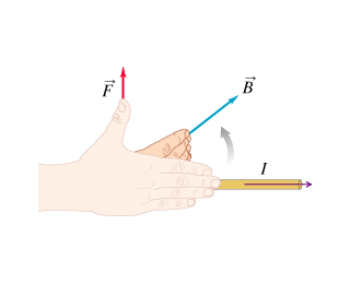
For notational reasons either lost to history or not worth looking up, the current (the direction the charge is moving) is I and the magnetic field is B. More reasonably, the Force the particle feels is F. In this case, the particle is moving to the right, but the magnetic field is going to make it curve upwards.
This works for positively charged particles (e.g., protons). If you’re wondering about negatively charged particles (electrons), then just reverse the direction you got. Or use your left hand. If the magnetic field stays the same, then eventually the ion will be pulled in a complete circle.
As it happens, the Earth has a magnetic field and the Sun fires charged particles at us (as well as every other direction) in the form of “solar wind”, so the right hand rule can explain most of what we see. The Earth’s magnetic field points from south to north through the Earth’s core, then curves around and points from north to south on Earth’s surface and out into space. So the positive particles flying at us from the Sun are pushed west and the negative particles are pushed east (right hand rule).
Since the Earth’s field is stronger closer to the Earth, the closer a particle is, the faster it will turn. So an incoming particle’s path bends near the Earth, and straightens out far away. That’s a surprisingly good way to get a particle’s trajectory to turn just enough to take it back into the weaker regions of the field, where the trajectory straightens out and takes it back into space. The Earth’s field is stronger or weaker in different areas, and the incoming charged particles have a wide range of energies, so a small fraction do make it to the atmosphere where they collide with air. Only astronauts need to worry about getting hit directly by particles in the solar wind; the rest of us get shrapnel from those high energy interactions in the upper atmosphere.
If a charge moves in the direction of a magnetic field, not across it, then it’s not pushed around at all. Around the magnetic north and south poles the magnetic field points directly into the ground, so in those areas particles from space are free to rain in. In fact, they have trouble not coming straight down. The result is described by most modern scientists as “pretty”.
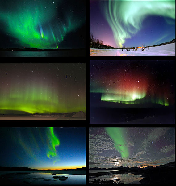
Charged particles from space following the magnetic field lines into the upper atmosphere where they bombard the local matter. Green indicates oxygen in the local matter.
The Earth’s magnetic field does more than just deflect ions or direct them to the poles. When a charge accelerates it radiates light, and turning a corner is just acceleration in a new direction. This “braking radiation” slows the charge that creates it (that’s a big part of why the aurora is inspiring as opposed to sterilizing). If an ion slows down enough it won’t escape back into space and it won’t hit the Earth. Instead it gets stuck moving in big loops, following the right hand rule all the way, thousands of miles above us (with the exception of our Antarctic readers). This phenomena is a “magnetic bottle”, which traps the moving charged particles inside of it. The doughnut-shaped bottles around Earth are the Van Allen radiation belts. Ions build up there over time (they fall out eventually) and still move very fast, making it a dangerous place for delicate electronics and doubly delicate astronauts.
Magnetic bottles, by the way, are the only known way to contain anti-matter. If you just keep anti-matter in a mason jar, you run the risk that it will touch the mason jar’s regular matter and annihilate. But ions contained in a magnetic bottle never touch anything. If that ion happens to be anti-matter: no problem. It turns out that the Van Allen radiation belts are lousy with anti-matter, most of it produced in those high-energy collisions in the upper atmosphere (it’s basically a particle accelerator up there). That anti-matter isn’t dangerous or anything. When an individual, ultra-fast particle of radiation hits you it doesn’t make much of a difference if it’s made of anti-matter or not.
And there isn’t much of it; about 160 nanograms, which (combined with 160 nanograms of ordinary matter) yields about the same amount of energy as 7kg of TNT. You wouldn’t want to run into it all in one place, but still: not a big worry.

A Van Allen radiation belt simulated in the lab.
In a totally unrelated opinion, this picture beautifully sums up the scientific process: build a thing, see what it does, tell folk about it. Maybe give it some style (time permitting).
The right hand picture is from here.


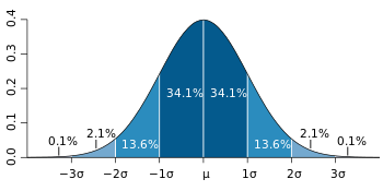
 excess wins or losses away from the average. For example, if you play 100 games, then
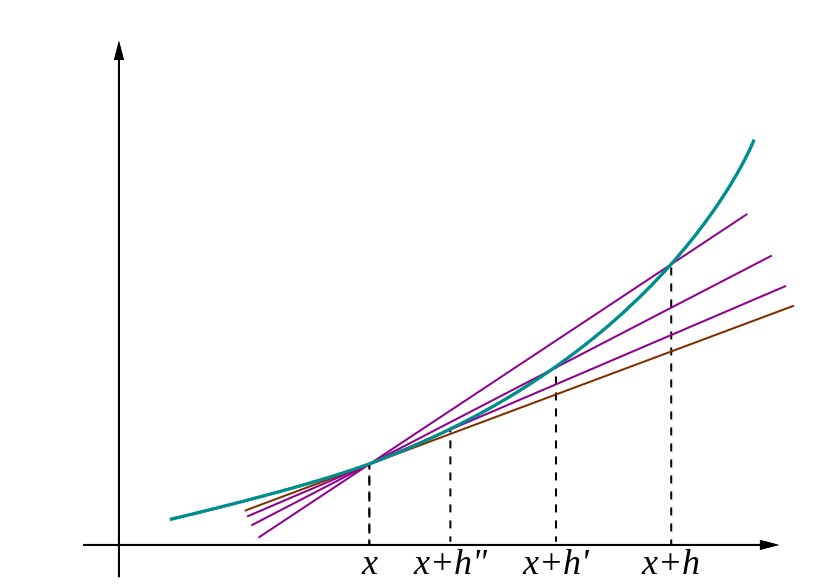
\right)") and
and \right)") is
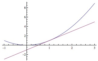
is -f(1)}{(1+h-1)}") and it just so happens that:
and it just so happens that:-f(1)}{(1+h-1)} \\= \frac{(1+h)^2-1^2}{h} \\= \frac{(1+2h+h^2)-1}{h} \\= \frac{2h+h^2}{h} \\= \frac{2h}{h}+\frac{h^2}{h} \\= 2+h\end{array}")
 is the easiest thing in the world: it’s 2. Exactly 2. Despite the fact that h=0 couldn’t be plugged in directly, there’s no problem at all. For every h≠0 you can draw a line between
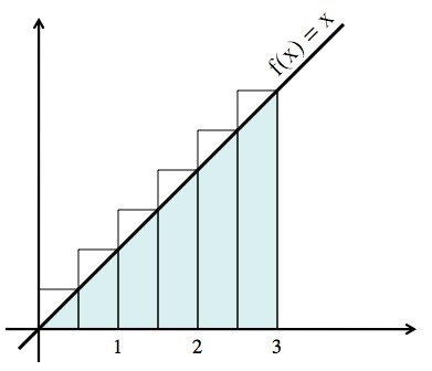
 or, in
 ") . If you add this up you get 5.25, which is more than 4.5 (the correct answer) because of those “sawteeth”. By using more rectangles these teeth can be made smaller, and the inaccuracy they create can be brought to naught. Here’s how!
. If you add this up you get 5.25, which is more than 4.5 (the correct answer) because of those “sawteeth”. By using more rectangles these teeth can be made smaller, and the inaccuracy they create can be brought to naught. Here’s how! wide and will be
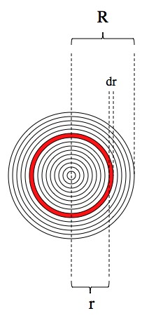
  tall (just so you can double-check, in the picture N=6). In mathspeak, the total area of these rectangles is
 \\ = \frac{3}{N}\frac{3}{N}\sum_{j=1}^N j \\ = \frac{9}{N^2}\sum_{j=1}^N j \\ = \frac{9}{N^2}\left(\frac{N^2}{2}+\frac{N}{2}\right) \\ = \frac{9}{2}+\frac{9}{2N} \\ \end{array}")
 is just one of those math things. For every finite value of N there’s an error of
  , but this can be made “arbitrarily small”. No matter how small you want the error to be, you can pick a value of N that makes it even smaller. Now, letting the number of rectangles “go to infinity”,
  and the correct answer is recovered: 9/2.
\frac{3}{N}")