Q: What would Earth be like if it didn’t turn?

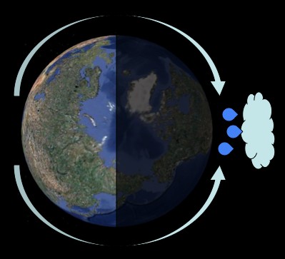
Physicist: The side of the Earth facing the sun would quickly become hotter than boiling water, and the side facing away would be cold enough for the atmosphere to freeze solid (condense into nitrogen and oxygen ice).  So all of the air and water would form glaciers of ice and what-was-once-air on the night side of the planet, and the day side of the planet would become an airless desert.  Without air to scatter sunlight, the sky would always be black, and the stars always visible.

Here I’m assuming that the Earth, rather than not rotating at all (which would result in one-year-long days), is in “phase lock” with the Sun the same way the Moon is in phase lock with the Earth.  So one side would always face the Sun and the other would always face away.

Air and water on the dark side of the earth would freeze. The Earth would be half desert, half water/air glaciers, and all atmosphere free.

We can estimate how hot and cold things would get by considering the Moon.  It’s the same distance from the Sun as the Earth is, so it’s a good test case.  Very quickly (within a few minutes) after the Sun rises at the beginning of the Moon’s 709 hour day the surface gets about as hot as it’s going to get: a balmy 110°C/230°F (give or take).

Some craters on the moon are never exposed to sunlight at all, which is exactly the situation the dark side of the Earth would be in, writ small.  They get as cold as -240°C/-400°F (that 30°C above absolute zero!).  That’s cold enough to freeze oxygen and nitrogen solid, even without air pressure.  So on the day side everything would get roasted, the oceans would evaporate out of their basins, and then drift to the dark side where they would form and condense onto massive glaciers.

For water at least, this is an effect already at work on our Earth (“spin Earth”?, “Rotopolis”?), it just doesn’t get very far.  That’s why (for example) the Antarctic ice cap is on average about as thick as the ocean is deep!

The non-rotating planet is a staple of sci-fi, and generally it’s declared that life could survive in the “twilight ring” between the day and night sides.  In fact, in the twilight ring the temperature would be colder than our poles are today (which are kinda like “twilight points”).  You find the “comfortable zone” about 20° into the day side from the ring.

Not that it matters.  What with the atmosphere being in such a state that you’d need a hammer and chisel to breathe, it wouldn’t be possible for life to exist anywhere.  The set up we have now is pretty good by comparison!

Posted in -- By the Physicist, Astronomy, Physics | 21 Comments

Q: According to the Many Worlds Interpretation, every event creates new universes. Where does the energy and matter for the new universes come from?

Physicist: There is no new energy or matter (or even new universes), it’s just that how it’s distributed depends on who’s asking, and in what “world” they’re doing the asking.  The important thing is: the universe doesn’t split or spawn new universes.

For those not familiar, here’s the crux of the problem.  If you don’t interact with (measure) things they behave like waves and can be in many places and do many things.  But when you do interact with a thing, it suddenly seems to only be in one state.  The double slit experiment is the classic example.  There are a couple of ways to explain this: the Copenhagen interpretation, psychic powers, Spaghetti Monsters, the Many World Interpretation, and a few others that are a little far-fetched.

If you go online (or read some kind of book or something) you generally find the Many Worlds Interpretation presented as the universe “splitting”.  Something along the lines of “everything that can happen will, just in different universes”.

From howstuffworks.com: “When a physicist measures the object, the universe splits into two distinct universes to accommodate each of the possible outcomes.”

From about.com: “…every time a ‘random’ event takes place, the universe splits between the various options available. Each separate version of the universe contains a different outcome of that event. Instead of one continuous timeline, the universe under the many worlds interpretation looks more like a series of branches splitting off of a tree limb.”

Quick aside: I’m about to talk about why this is wrong, but don’t take that as a criticism.  The “splitting/branching” thing is about the only narrative anyone ever hears, so I’m not knocking the fine and hard-working people of “about” and “howstuffworks” (or the authors of the hundreds of other examples out there).  Much respect.

So, supposedly every time any kind of quantum event happens that could have one of several results (which is essentially every moment for every thing, which is plenty) the entire freaking universe splits into many universes.  But, the universe contains a lot of energy.  Like, even more than the U.S. uses in a year.  So, whence does this energy come?

First off, in a not-really-explaining-anything nutshell: the universe doesn’t branch so much as it meanders and intertwines.  This isn’t an answer to the energy question, but it’s worth mentioning.

If you want a picture to work with, rather than thinking about the universe as an ever-branching tree, think of it as an intertwining (albeit, very complex) rope.

The many (like: many, many) different versions of the universe branch apart, and come together all over the place.  That is; one event can certainly lead to several outcomes, but in the same way, several causes can lead to the same event.  Everything the could happen will happen (given the present) and everything that could have happened did happen (given the present).  You can think of this as un-branching, or branching into the past.  Either way.  The Franson experiment, which demonstrates a single photon emitted at two different times in the past interfering with itself (isn’t that weird?), is one of the most beautiful examples of this “backward branching”.

That doesn’t answer the question, but it does sorta help set the stage for the universe being more complicated than just “splitting”.

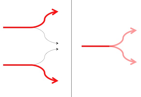
The way that energy is conserved depends on the context of the question.  Say you’ve got a particle and at some point, for whatever reason, it finds that it has to take one of two paths.  There are a lot of reasons this could happen, but the particulars aren’t important.  The cases to consider are: 1) you measure it taking one of the two paths and 2) you don’t.

Although the details change, the total amount of energy stays constant from all perspectives. Both from inside the system (left) where all the energy is concentrated on one of the possible paths, as well as when seen from outside (right) in which the particle and its associated energy can be distributed among the different paths.

If you’re “caught up” with the particle in question, maybe by observing it / interacting with it, you find that it only takes one path (More accurately, each of the different versions of you see each of the different versions of the particle taking one path).  You’ll see the particle start out, “choose” between the upper and lower paths (a random choice), and continue on.  From your perspective the total energy never changes.  You may have a sneaking suspicion that there are other quantum worlds, but you never (none of your versions ever) actually see a problem.  To have a problem you’d need to be able to see more than one of the particle’s “worlds”.

But that’s no problem!  Seeing a particle in multiple states (each of which is a different “world” to the particle) is the oldest trick in the quantum book. This, by the way, is one of the great weakness of the language involved.  You’d think that “worlds” and “universes” would have to be completely separate.  But while the different states of the particle each see each other as being in different worlds, for something that sees the super-position of all those states (for example, something that sees the interference fringes in the double slit experiment) they seem to be in the same world.

When a particle (or whatever) is in multiple states its energy and matter is distributed among those various states.  In the two-equally-probable-paths example above, half of particle’s existence takes one path and half takes the other.  Likewise, its energy and matter are divided among the paths.

Although you can’t measure “half a particle” (a particle’s nature is to be indivisible), you can show that particles often need to be in multiple states (so their existence can be spread out), and you can even calculate and measure how much of each particle must be taking various paths.  Again, the double slit experiment is an excellent example.

So, in the two-path example, a particle comes along with some amount of energy.  When it has a choice of two paths it takes both.  The energy of the particle is divided in proportion to the probability of the path taken.  So, for example, 50% chance of each path means equal division of the energy and matter of the particle.  Before the fork all of the energy is on one path, and afterwards, despite the fact that the particle is behaving as though it’s in two places, the same amount of energy is present, just spread out.

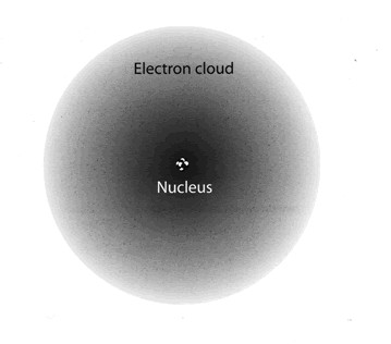
It may seem deeply weird to say that, but you could argue that no particle keeps all its matter/energy/existence in one place at a time.  For example, if you look at an electron in an atom you find that it’s smeared out around the nucleus in the form of an “electron cloud”.  Electrons don’t orbit atoms like planets around the Sun, they “wave” around the nucleus like vibrations in a ringing bell.

That, and other terrible similes, will be included in my upcoming book, “some thing are like these other things, but different, y’know?: a book that’s like a collection of similes”.

Each electron in an atom forms a "cloud" around the nucleus. Literally, it is in every possible position (some more than others). The nucleus itself takes the form of proton and neutron clouds, they're just much, much smaller.

For “uncertainty principle” type reasons, electrons (and everything else) always exist in a “cloud” of locations, all at once.  You can say “there is an electron around this atom” and you can say “the energy and matter of the electron is around this atom”, but there’s nothing you can say past that.  The existence of the electron, and everything else about it, is spread out.

Each different version of a thing, and every “parallel world” may see itself as holding all of its energy and matter, but from an outside perspective (where the “many-worldness” becomes important) it’s just part of a greater whole.  Either way, energy is always conserved.  So, while it’s fun to talk about “other quantum realities” and “different universes”, it’s more accurate to say that everything is happening in one universe.  One, stunningly complex, weirdly put together, entirely counter-intuitive universe.

Posted in -- By the Physicist, Physics, Quantum Theory | 44 Comments

Q: Can wind chill make things “feel” colder than absolute zero?

The original question was: Is it possible for something to “feel” colder than absolute zero?  If the forecast called for 1K (1 Kelvin) with 20mph gusts of wind, would the wind chill be below 0K?


Physicist: This is a beautiful question!

Wind chill” is a very ad hoc, artificial measure used to describe the fact that cold air pulls heat out of us faster when it’s moving.

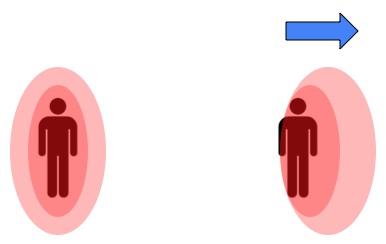
When air is stagnant and you’re standing still, you’ll be surrounded by a bubble of warm air (heated by body heat).  This bubble insulates us from the surrounding air temperature.  So, if it’s 40°F out, and there’s no wind, you’ll actually be losing heat as though it were warmer, because near your body it is warmer.  In fact, this is the whole point of clothes (beyond the whole modesty thing): keeping a layer of air near the body.  The insulation provided by the cloth is generally dwarfed by the insulation provided by the air it holds in.

So, when you walk outside and say “it feels like it’s about 70°F out” what you really mean is “the bubble of air around me feels like it’s about 85°F, and my experience tells me that corresponds to an ambient temperature of 70°F”.  But you’d need to be kind of a jerk to go through all that.  Instead you just say “feels like 70°F” (even though what you’re experiencing is actually warmer).

When the wind is blowing however, that layer of warm air is pushed away and we’re exposed to the actual air temperature.  What we call the wind chill temperature is the temperature it would have to be in order for you to lose body heat at the same rate, were the air to be sitting still.

Being not just squishy but warm as well, we heat up the air immediately around our bodies. This air insulates us from direct exposure to the surrounding cold air. When there's wind that bubble gets thinner and with less insulation we lose heat faster. This picture is not to scale, and is a poor representation to boot.

Wind chill is pretty subjective (people of different sizes and shapes will experience wind chill differently), and not terribly exact, but the standard gives you a decent ball park estimate.

If you were to stick your hand into liquid helium at 1K, you would again get a layer of slightly warmer liquid helium around your hand (I’m using liquid helium here because it stays liquid essentially all the way to 0).  If you were to stick your hand in flowing liquid helium, that warmer layer would be washed away and your hand would be exposed to actual 1K helium.

As strange as it sounds, it is perfectly fair to say that, with “wind chill”, the temperature is below 0K, because that’s how cold stagnant helium would have to be to match the heat loss caused by 1K helium that’s moving.

There’s nothing wrong with this statement.  Heat loss is governed by the difference in temperature between a body and its environment.  Regardless of whether or not one of the temperatures involved is below zero.

Posted in -- By the Physicist, Physics | 10 Comments

Q: What is “spin” in particle physics? Why is it different from just ordinary rotation?

Physicist: “Spin” or sometimes “nuclear spin” or “intrinsic spin” is the quantum version of angular momentum.  Unlike regular angular momentum, spin has nothing to do with actual spinning.

Normally angular momentum takes the form of an object’s tendency to continue rotating at a particular rate.  Conservation of regular, in-a-straight-line momentum is often described as “an object in motion stays in motion, and an object at rest stays at rest”, conservation of angular momentum is often described as “an object that’s rotating stays rotating, and an object that’s not rotating keeps not rotating”.

Any sane person thinking about angular momentum is thinking about rotation.  However, at the atomic scale you start to find some strange, contradictory results, and intuition becomes about as useful as a pogo stick in a chess game.  Here’s the idea behind one of the impossibilities:

Anytime you take a current and run it in a loop or, equivalently, take an electrically charged object and spin it, you get a magnetic field.  This magnetic field takes the usual, bar-magnet-looking form, with a north pole and a south pole.  There’s a glut of detail on that over here.
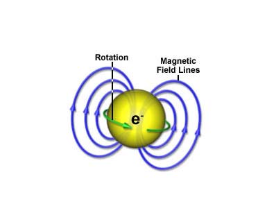
A spinning charged object carries charge in circles, which is just another way of describing a current loop. Current loops create “dipole” magnetic fields.

If you know how the charge is distributed in an object, and you know how fast that object is spinning, you can figure out how strong the magnetic field is.  But in general, more charge and more speed means more magnetism.  Happily, you can also back-solve: for a given size, magnetic field, and electric charge, you can figure out the minimum speed that something must be spinning.
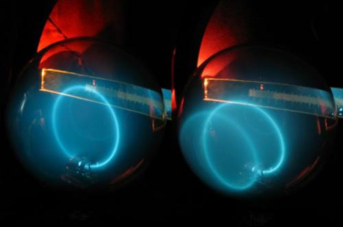
It’s not too hard to find the magnetic field of electrons, as well as their size and electric charge. Btw, these experiments are among the prettiest experiments anywhere.  Suck on that biology!

Electrons do each have a magnetic field (called the “magnetic moment” for some damn-fool reason), as do protons and neutrons.  If enough of them “agree” and line up with each other you get a ferromagnetic material, or as most people call them: “regular magnets”.

Herein lies the problem.  For the charge and size of electrons in particular, their magnetic field is way too high.  They’d need to be spinning faster than the speed of light in order to produce the fields we see.  As fans of the physics are no doubt already aware: faster-than-light = no.  And yet, they definitely have the angular momentum necessary to create their fields.

It seems strange to abandon the idea of rotation when talking about angular momentum, but there it is.  Somehow particles have angular momentum, in almost every important sense, even acting like a gyroscope, but without doing all of the usual rotating.  Instead, a particle’s angular momentum is just another property that it has, like charge or mass.  Physicists use the word “spin” or “intrinsic spin” to distinguish the angular momentum that particles “just kinda have” from the regular angular momentum of physically rotating things.

Spin (for reasons that are horrible, but will be included anyway in the answer gravy below) can take on values like \cdots, , -\hbar, -\frac{1}{2}\hbar, 0, \frac{1}{2}\hbar, \hbar, \frac{3}{2}\hbar, \cdots where \hbar (“h bar“) is a physical constant.  This by the way, is a big part of where “quantum mechanics” gets its name.  A “quantum” is the smallest unit of something and, as it happens, there is a smallest unit of angular momentum (\frac{1}{2}\hbar)!

It may very well be that intrinsic spin is actually more fundamental than the form of rotation we’re used to.  The spin of a particle has a very real effect on what happens when it’s physically rotated around another, identical particle.  When you rotate two particles so that they change places you find that their quantum wave function is affected.  Without going into too much detail, for particles called fermions this leads to the “Pauli Exclusion principle” which is responsible for matter not being allowed to be in the same state (which includes place) at the same time.  For all other particles, which are known as “bosons”, it has no effect at all.


Answer gravy: Word of warning; this answer gravy is pretty thick.  A familiarity with vectors, and linear algebra would go a long way.

Not everything in the world commutes.  That is, AB≠BA.  In order to talk about how badly things don’t commute physicists (and other “scientists”) use commutators.  The commutator of A and B is written “[A,B] = AB-BA”.  When A and B don’t commute, then [A,B]≠0.

As it happens, the position measure in a particular direction, Rj, doesn’t commute with the momentum measure in the same direction, Pj (“j” can be the x, y, or z directions).  That is to say, it matters which you do first.  This is more popularly talked about in terms of the “uncertainty principle“.  On the other hand, momentum and position measurements in different directions commute no problem.

For example, [R_x,P_x]=i\hbar and [R_x,P_y]=0.  This is more succinctly written as [R_j,P_k]=i\hbar \delta_{jk}, where \delta_{jk}=\left\{\begin{array}{ll}1&when\,j=k\\0&when \,j\ne k\end{array}\right.  This is the “position/momentum canonical commutation relation“.

In both classical and quantum physics the angular momentum is given by \vec{R}\times\vec{P}.  This essentially describes angular momentum as the momentum of something (\vec{P}) at the end of a lever arm (\vec{R}).  Classically \vec{R} and \vec{P} are the position and momentum of a thing.  Quantum mechanically they’re measurements applied to the quantum state of a thing.

For “convenience”, define the “angular momentum operator”, \vec{L}, as \hbar\vec{L}=\vec{R}\times\vec{P} or equivalently \hbar\vec{L}_\ell=\sum_{jk}\epsilon_{jk\ell}\vec{R}_j\vec{P}_k, where \epsilon_{jk\ell} is the “alternating symbol“.  This is just a more brute force way of writing the cross product.

Now check this out!  (the following uses identities from here and here)

\begin{array}{ll}\hbar^2[L_j,L_k]\\=[\hbar L_j,\hbar L_k]\\=\left[\sum_{st}\epsilon_{stj}\vec{R}_s\vec{P}_t, \sum_{mn}\epsilon_{mnk}\vec{R}_m\vec{P}_n\right]\\=\sum_{stmn}\epsilon_{stj}\epsilon_{mnk}\left[\vec{R}_s\vec{P}_t,\vec{R}_m\vec{P}_n\right]\\=\sum_{stmn}\epsilon_{stj}\epsilon_{mnk}\left(\left[\vec{P}_t,\vec{R}_m\right]\vec{R}_s\vec{P}_n+\left[\vec{P}_t,\vec{P}_n\right]\vec{R}_s\vec{R}_m+\left[\vec{R}_s,\vec{R}_m\right]\vec{P}_t\vec{P}_n+\left[\vec{R}_s,\vec{P}_n\right]\vec{P}_t\vec{R}_m\right)\\=\sum_{stmn}\epsilon_{stj}\epsilon_{mnk}\left(-i\hbar\delta_{tm}\vec{R}_s\vec{P}_n+0+0+i\hbar\delta_{sn}\vec{P}_t\vec{R}_m\right)\\=i\hbar\sum_{stmn}\epsilon_{stj}\epsilon_{mnk}\left(\delta_{sn}\vec{P}_t\vec{R}_m-\delta_{tm}\vec{R}_s\vec{P}_n\right)\\=i\hbar\sum_{stmn}\epsilon_{stj}\epsilon_{mnk}\delta_{sn}\vec{R}_m\vec{P}_t-i\hbar\sum_{stmn}\epsilon_{stj}\epsilon_{mnk}\delta_{tm}\vec{R}_s\vec{P}_n\\=i\hbar\sum_{stm}\sum_n\epsilon_{stj}\epsilon_{mnk}\delta_{sn}\vec{R}_m\vec{P}_t-i\hbar\sum_{stn}\sum_m\epsilon_{stj}\epsilon_{mnk}\delta_{tm}\vec{R}_s\vec{P}_n\end{array} \begin{array}{ll}=i\hbar\sum_{stm}\epsilon_{stj}\epsilon_{msk}\vec{R}_m\vec{P}_t-i\hbar\sum_{stn}\epsilon_{stj}\epsilon_{tnk}\vec{R}_s\vec{P}_n\\=i\hbar\sum_{tm}\left(\sum_s\epsilon_{stj}\epsilon_{msk}\right)\vec{R}_m\vec{P}_t-i\hbar\sum_{sn}\left(\sum_t\epsilon_{stj}\epsilon_{tnk}\right)\vec{R}_s\vec{P}_n\\=i\hbar\sum_{tm}\left(\delta_{tk}\delta_{jm}-\delta_{tm}\delta_{jk}\right)\vec{R}_m\vec{P}_t-i\hbar\sum_{sn}\left(\delta_{sk}\delta_{jn}-\delta_{sn}\delta_{jk}\right)\vec{R}_s\vec{P}_n\\=i\hbar\sum_{tm}\delta_{tk}\delta_{jm}\vec{R}_m\vec{P}_t-i\hbar\sum_{tm}\delta_{tm}\delta_{jk}\vec{R}_m\vec{P}_t-i\hbar\sum_{sn}\delta_{sk}\delta_{jn}\vec{R}_s\vec{P}_n+i\hbar\sum_{sn}\delta_{sn}\delta_{jk}\vec{R}_s\vec{P}_n\\=i\hbar\vec{R}_j\vec{P}_k-i\hbar\sum_{t}\delta_{jk}\vec{R}_t\vec{P}_t-i\hbar\vec{R}_k\vec{P}_j+i\hbar\sum_{s}\delta_{jk}\vec{R}_s\vec{P}_s\\=i\hbar\vec{R}_j\vec{P}_k-i\hbar\vec{R}_k\vec{P}_j\\=i\hbar^2\epsilon_{jk\ell}L_{\ell}\end{array}

Therefore: [L_j,L_k]=i\epsilon_{jk\ell}L_{\ell}.

So what was the point of all that?  It creates a relationship between the angular momentum in any one direction, and the angular momenta in the other two.  Surprisingly, this allows you to create a “ladder operator” that steps the total angular momentum in a direction up or down, in quantized steps.  Here are the operators that raise and lower the angular momentum in the z direction:

\begin{array}{ll}L_+ = L_x+iL_y\\L_- = L_x-iL_y\\\end{array}

Notice that

\begin{array}{ll}[L_z,L_+]\\=[L_z,L_x\pm iL_y]\\=[L_z,L_x]\pm i[L_z,L_y]\\=iL_y\pm i(-iL_x)\\=iL_y\pm L_x\\=\pm(L_x \pm iL_y)\\=\pm L_\pm\end{array}

Here’s how we know they work.  Remember that Li is a measurement of the angular momentum in the “j” direction (any one of x, y, or z).  For the purpose of making the math slicker, the value of the angular momentum is the eigenvalue of the L operator.  If you’ve made it this far; this is where the linear algebra kicks in.

Define the “eigenstates” of Lz, |m\rangle, as those states such that L_z|m\rangle=m|m\rangle.  “m” is the amount of angular momentum (well… “m\hbar” is), and |m\rangle is defined as the state that has that amount of angular momentum.  Now take a look at what (for example) L_+ does to |m\rangle:

\begin{array}{ll}L_zL_+|m\rangle\\=\left(L_zL_+-L_+L_z+L_+L_z\right)|m\rangle\\=\left([L_z,L_+]+L_+L_z\right)|m\rangle\\=[L_z,L_+]|m\rangle+L_+L_z|m\rangle\\=L_+|m\rangle+L_+L_z|m\rangle\\=L_+|m\rangle+mL_+|m\rangle\\=(1+m)L_+|m\rangle\end{array}

Holy crap!  L_+|m\rangle is an eigenstate of L_z with eigenvalue 1+m.  This is because, in fact, L_+|m\rangle = |m+1\rangle!

Assuming that there’s a maximum angular momentum in any particular direction, say “j”, then the states range from |-j\rangle to |j\rangle in integer steps (using the raising and lowering operators).  That’s just because the universe doesn’t care about the difference between the z and the negative z directions.  So, the difference between j and negative j is some integer: j-(-j) = 2j = “some integer”.  For ease of math the \hbar were separated from the L’s in the definition.  The actual angular momentum is “j\hbar“.

By the way, notice that at no point has mass been mentioned!  This result applies to anything and everything.  Particles, groups of particles, your mom, whatevs!

So, the maximum or minimum angular momentum is always some multiple of half an integer.  When it’s an integer (0, 1, 2, …) you’ve got a boson, and when it’s not (1/2, 3/2, …) you’ve got a fermion.  Each of these types of particles have their own wildly different properties.  Most famously, fermions can’t be in the same state as other fermions (this leads to the “solidness” of ordinary matter), while bosons can (which is why light can pass through itself).

Notice that the entire ladder operator thing for any L_j is dependent on the L operators for the other two directions.  In three or more dimensions you have access to at least two other directions, so the argument holds and particles in 3 or more dimensions are always fermions or bosons.

In two dimensions there aren’t enough other directions to create the ladder operators (L_\pm).  It turns out that without that restriction particles in two dimensions can assume any spin value (not just integer and half-integer).  These particles are called “anyons”, as in “any spin”.  While actual 2-d particles can’t be created in our jerkwad 3-d space, we can create tiny electromagnetic vortices in highly constrained, flat sheets of plasma that have all of the weird spin properties of anyons.  As much as that sounds like sci-fi, s’not.

It’s one of the several proposed quantum computer architectures that’s been shown to work (small scale).
Posted in -- By the Physicist, Equations, Math, Particle Physics, Physics, Quantum Theory | 77 Comments

Q: What is Bayes’ rule and how do I use it to improve my life?

Mathematician: Bayes’ theorem in one of the most practically useful equations coming from the field of probability. If you take its implications to heart it will make you better at figuring out the truth in a variety of situations. What makes the rule so useful is that it tells you what question you need to ask to evaluate how strong a piece of evidence is. In my own life, I apply this concept nearly every week.

Let’s consider an example. Suppose you have a cough that’s been going on for days, and you’re not sure what’s causing it. You believe it could be caused by allergies (we’ll call this hypothesis A), or by a bronchitis (which we’ll call hypothesis B).

Now, let’s suppose that you take an anti-allergy medication, and for the next hour your cough disappears. We can view this occurrence as evidence, which we should expect to have a bearing on how much more likely A is than B. But how strong is this evidence, and how do we rigorously show which of our hypotheses it supports? Bayes’ rule tells us that the answer lies in the Bayes Factor, which is the answer to the following question:

“How much more likely would it have been for this evidence to occur if A were true than if B were true?”

This question completely captures how strongly the evidence supports A compared to B. It must lead to one of three conclusions:

  1. The evidence would have been more likely to occur if A were true than if B were true. This implies the evidence supports A rather than B.
  2. The evidence would be just as likely to occur if A were true as if B were true. This implies the evidence has no bearing on the question of whether A or B is more probable. Hence,  the “evidence” isn’t really evidence at all when it comes to evaluating the relative likelihood of these two hypothesis.
  3. The evidence would have been more likely to occur if B were true than if A were true. This implies the evidence supports B rather than A.

In our cough example, the Bayes factor becomes the answer to the question:

“How much more likely would it be for my cough to disappear for an hour after taking an anti-allergy medication if I was suffering from allergies compared to if I had bronchitis?”

You can estimate this value in a rough way. Anti-allergy medication should have essentially no effect on coughs from bronchitis. It is possible that you have bronchitis and your cough just happened to go away by chance during this particular hour, but that is unlikely (certainly less likely than 1 in 10 for a long lasting, consistent cough). On the other hand, allergy medication tends to be fairly effective against coughs caused by allergies, so we should expect there to be at least a 1 in 3 chance that your cough would go away after taking the medication if you did in fact have allergies. Hence, in this case we can produce a conservatively low estimate for the Bayes factor with just a couple minutes of thought. How likely the cough was to have stopped given A we put at least at 1/3. How likely the cough was to stop given B we put at most at 1/10. Hence, the Bayes Factor, which is how likely the cough was to stop given A compared to how likely it was to stop given B, is greater than (1/3) / (1/10) = 3.3.

This should be interpreted as saying that we should now believe A is at least 3.3 times more likely compared to B than we used to think it was. In other words, the Bayes Factor tells us how much our new evidence should cause us to update our belief about the relatively likelihood of our two hypothesis. However many times more likely we thought A was than B before evaluating this anti-allergy medication evidence, we should update this number by multiplying by the Bayes factor. The result will tell us how much more likely A is than B having taken into account both our prior belief and the new information.

Now suppose that (since you get coughs caused by allergies a lot more often than you get bronchitis) you thought it was 4 times more likely that A was true than B before you took the anti-allergen. You now have more evidence, since you saw that the cough disappeared after taking the medicine. You’ve already calculated that the Bayes Factor is at least 3.3. All we have to do now is adjust our prior belief (that A was 4 times more likely than B) by multiplying by the Bayes Factor. That means you should now believe A is at least 13.3 = 3.3 * 4 times more likely than B.

Bayes’ rule is remarkably useful because it tells us the right question to ask ourselves when evaluating evidence. If we are considering two hypotheses, A and B, we should ask “how much more likely would this evidence have been to occur if A were true than if B were true?” On the other hand, if we just are evaluating one hypothesis, and we want to know whether evidence makes it more or less likely, we can replace B with “not A” and phrase the question as “how much more likely would this evidence have been to occur if A were true compared to if A were not true?” The answer to this question, which is the Bayes Factor for this problem, completely captures the strength of the evidence with regard to A. If the answer is much greater than 1, then the evidence strongly supports A. If the Bayes Factor is slightly bigger than 1, it slightly supports A. If it is precisely 1, the evidence has no bearing on A (i.e. the “evidence” doesn’t actually provide evidence with respect to A). If it is slightly below 1, it should slightly reduce your credence in A. If it is substantially below 1, it should substantially decrease your belief in A.

Unfortunately, the human brain does not always deal with evidence properly. Our intuition about what is, or is not evidence, and what is strong versus weak evidence, can be terribly wrong (see, for instance, the base rate fallacy). However, by thinking in terms of the Bayes factor, we can check our intuition, and use evidence much more effectively. We can avoid many thinking errors and biases. We simply need to get in the habit of asking, “How much more likely would this evidence have been to occur if A were true than if B were true?”

Worried that someone doesn’t like you because he hasn’t returned your phone call in two days? Ask, “how much more likely would this be to occur if he liked me than if he didn’t like me?”

Believe that “an absence of evidence for A is not evidence of absence of A”? Ask, “how much more likely would this absence of evidence for A be to occur if A were not true versus if A were true?”

Think that the stock you bought that went up 30% is strong evidence for you having skill as an investor? Ask, “how much more likely is it that my highest returning stock pick would go up 30% if I was an excellent investor compared to if I was just picking stocks at random?”


Proof:

Now, let’s break out some math to prove that what we’ve said is right. We’ll use P(A) to represent the probability you assigned to hypothesis A being true before you saw the latest evidence. We’ll use E to refer to the new evidence. We’ll let P(A|E) be the probability of A given that you’ve seen the evidence E, and P(A,E) will be the probability of both A and E occurring. Now, by definition, we have that:

P(A|E) = \frac{P(A, E)}{P(E)}.

The intuitive explanation behind this definition comes from observing that the probability of A when we know E (the left hand side) should be the same as how often both A and E are true compared to how often just E is true (the right hand side). Now, we can reuse this definition, but this time for P(E|A). This gives us:

P(E|A) = \frac{P(A, E)}{P(A)}.

Rearranging so that the last two expressions give P(A,E) alone on one side of the equation, and then setting them equal to each other, we get:

P(A|E) P(E) = P(E|A) P(A).

Dividing both sides by P(E) yields the typical representation of Bayes’ rule:

P(A|E) = \frac{P(E|A) P(A)}{P(E)}.

Now, we can write the same expression but replace our first hypotheses A with our second hypotheses B. This yields Bayes’ rule for B:

P(B|E) = \frac{P(E|B) P(B)}{P(E)}.

Dividing the expression for P(A|E) by the expression for P(B|E) we get:

\frac{P(A|E)}{P(B|E)} = (\frac{P(E|A)}{P(E|B)}) (\frac{P(A)}{P(B)})

In words, this says that how much more likely A is than B after evaluating our evidence, which is the left side of our equation, is equal to the product of the two factors on the right. The second factor on the right is how much more likely A was than B before we saw our evidence. This reflects our “prior” belief about A and B. The first factor on the right is the Bayes Factor, which “updates” our prior belief to incorporate the new evidence. The Bayes Factor just says how much more likely the evidence would be to occur if A were true than if B were true. To summarize: how much more likely A is than B now is just equal to how much more likely A was than B before we saw our new evidence, times how much more likely this evidence would be to occur if A were true than if B were true.

If, rather than comparing two hypotheses, we want to just update our belief about the single hypothesis A, we can do this by substituting the event “not A”, written \overline A, for the event B. Then, our formula reads:

\frac{P(A|E)}{P(\overline A|E)} = (\frac{P(E|A)}{P(E|\overline A)}) (\frac{P(A)}{P(\overline A)}).

Posted in -- By the Mathematician, Equations, Math, Probability | 8 Comments

Q: Are there universal truths?

Physicist: That something exists, that it is more complex than trivially simple, and it includes me (cogito ergo sum, and all that).

It doesn’t seem like you can say much more.  At least, this brain-in-a-box can’t.


Philosopher: Depends on what you mean by ‘universal’.

One option:  not subject-relative.  I.e., not like “seaweed stir-fry is tasty” which seems true to me but not to my undergraduates.  Then we have a whole host of universal truths.  2+2=4, polar bears eat fish, there was an earthquake in Los Angeles in September of 2011, and (I think) torturing puppies for fun is immoral.

Another option:  necessarily true.  Then we just have the truths that couldn’t be otherwise.  Math still counts, but maybe Physics truths don’t.  Truths of Logic definitely count.  So do truths like: nothing can be red all over and green all over.

Finally, one might mean:  fundamental truths.  Presumably these would include mathematical, physical, and metaphysical laws.  (E.g., for a metaphysical law:  for any x, y, and z, if x is part of y, and y is part of z, then x is part of z.)

Posted in -- By the Physicist, -- Guest Author, Philosophical | 8 Comments