Q: Do we have free will?

Physicist: If you want to get into an argument that drags on forever, you can frame a question like this in terms of consciousness, and the nature of choice, or any number of other ill-defined ill-understood ideas.  So consider only the question in terms of determinism;

Q: “does the state of the universe now (and in the past) completely determine the future of the universe and, by inclusion, the future of me?”

Back in the day (classical physics day) the answer could rightly be “yes” or “I don’t know”.  However, with the advent of modern quantum mech we’ve managed to make great strides on questions like this.  Now we can answer: “yes, no, and kinda”!  It’s progress like this that almost makes going back to clipper ships and horse carts worth it.

One of the biggest weirdnesses to come out of quantum mechanics is the idea of “super-position”, which is that a single thing (a particle or whatever) can be in multiple states at the same time (the state of a thing can involve position, speed, orientation, and even how the thing is related to other things).  QM allows us to see how all of those states change in time and interact each other.  However, any direct interaction with an “undetermined state” will reveal it to be in only one (of its many) state(s).  In what follows I’ll use “universe” to mean the universe with just one state (things did happen this way), and multiverse to mean all the states involved simultaneously (with all the interference and what-have-you).

The two ways of looking at this are the “Copenhagen interpretation” (wrong) and the “many worlds interpretation” (right).

“Yes!”: Given complete knowledge of the multiverse’s quantum wave function you can determine the future of that function forever.  Unfortunately, this isn’t particularly useful for those of us who live inside the universe.  The wave function in question encompasses all possibilities simultaneously and involves plenty of self-interference.  For example: when you do the double slit experiment you can calculate exactly what the fringes will look like on the screen, by doing a calculation that assumes that the photons involved go through both slits.  However, if you were to instead look a one of the slits, this doesn’t tell you anything about whether or not you will see the photon go through that slit.

(Just a quick note about the link above.  “The Secret”, and its creepy brainchild “What the bleep”, are both symptoms of a greater douchiness, but despite their culty bent they explain the double slit pretty well.)

In fact what happens is it goes through both slits, but in turn there are different versions of you that see both outcomes.  If you look at the multiverse as a whole (seeing every state) then everything is completely deterministic.  If you look at just one tiny piece at a time (like we seem to), then everything seems random.

Essentially, for every choice you can make, there are a whole mess of versions of you (identical up to the moment of choice) that do make that choice.  In fact, if your wave function is known completely, then how much (many?) of you goes down any road can be derived.  I don’t want to hear anyone saying “but I chose to do that!”, because some (part?) of you had to.  But then, some of you had to do every available choice.

“No!”: Part of the Copenhagen interpretation is fundamental, true randomness.  There’s no multiverse in Copenhagen (so don’t go flying there to look), so any choice you make is unpredictable (or at least, not completely predictable, there are some pretty reliable people out there) in the sense that no matter how good your fore-knowledge of someone’s wave function, you still can’t make perfect predictions.

It’s seems like there’s enough wiggle room in there to fit some free will.

“Kinda!”: Even if you subscribe to the many world hypothesis you could argue that “dude, who cares?”.  You’ll never meet (can’t meet) those other versions of yourself, so what does it matter that, in theory, all of your simultaneous actions are determined in a multiverse-kind-of-way?  Doesn’t.

Posted in -- By the Physicist, Paranoia, Philosophical, Physics, Quantum Theory | 13 Comments

Q: How did mathematicians calculate trig functions and numbers like pi before calculators?

Physicist: Don’t know.  But if you’re ever stuck on a desert island, here are some tricks you can use.  The name of the game is “Taylor polynomials“.

\sin{(x)} = \sum_{n=0}^\infty \frac{(-1)^n}{(2n+1)!} x^{2n+1} = \frac{x}{1} - \frac{x^3}{1 \cdot 2 \cdot 3} + \frac{x^5}{1 \cdot 2 \cdot 3 \cdot 4 \cdot 5} - \frac{x^7}{1 \cdot 2 \cdot 3 \cdot 4 \cdot 5 \cdot 6 \cdot 7} + \cdots \cos{(x)} = \sum_{n=0}^\infty \frac{(-1)^n}{(2n)!} x^{2n} = 1 - \frac{x^2}{1 \cdot 2} + \frac{x^4}{1 \cdot 2 \cdot 3 \cdot 4} - \frac{x^6}{1 \cdot 2 \cdot 3 \cdot 4 \cdot 5 \cdot 6} + \cdots

All the other trig function are just combinations of sine and cosine, so this is really all you need.  Of course, you can’t add up an infinite number of terms, so if you only go up to the xL term then the error between the sum you have and the actual value of sine or cosine is no more than \frac{x^L}{L!}.  Now x can be pretty big, but you can use the fact that sine and cosine repeat every 2 \pi, as well as the fact that \sin{(x \pm \pi)} = -\sin{(x)} and \cos{(x \pm \pi)} = -\cos{(x)}, to get the “x” down to -\frac{\pi}{2} \le x \le \frac{\pi}{2}.  So if you sum up to the xL term, then your error will be no larger than \frac{1}{L!} \left( \frac{\pi}{2} \right)^L.  The “1/L!” makes this error pretty small.  Summing up to the x10 term will be accurate to within 3 parts in 100,000 at worst.

For example:

\sin{(16)} = \sin{(16 - 2\pi)} = \sin{(16 - 4\pi)} = -\sin{(16 - 5\pi)} \approx -\sin{(0.2920)}

Summing up to the x5 term yields:

\sin{(16)} \approx -\sin{(0.2920)} \approx - \left( 0.2920 - \frac{0.2920^3}{6} + \frac{0.2920^5}{120} \right) = - 0.2879

Which is accurate to at least the first 4 decimal places.

There aren’t a hell of a lot of important mathematical constants out there.  The most important are “e” and “\pi“.

e^x = \lim_{m \to \infty} \left( 1 +\frac{x}{m} \right)^m \approx \sum_{n=0}^L \frac{x^n}{n!} = 1+ \frac{x}{1}+\frac{x^2}{1 \cdot 2}+\frac{x^3}{1 \cdot 2 \cdot 3}+\cdots with an error of no more than \frac{x^{L+1}}{(L+1)!}.  This is another example of a Taylor polynomial.  To calculate only e, just set x=1.

\pi \approx 4 \sum_{n=0}^L \frac{(-1)^n}{2n+1} = 4 \left( 1 - \frac{1}{3} +\frac{1}{5} - \frac{1}{7} + \cdots \right) with an error of no more than \frac{4}{2L+3}.  One way to derive this equation is to take the Taylor series for Arctan, and plug in 1 (\arctan{(1)} = \frac{\pi}{4}).  This is easy to remember but slow to converge (2,000 terms to get 3 decimal places), so here’s a better one:

\pi \approx \sqrt{12}\sum^L_{k=0} \frac{(-1)^k}{(2k+1) 3^k} = \sqrt{12}\left(1-{1\over 3\cdot3}+{1\over5\cdot 3^2}-{1\over7\cdot 3^3}+\cdots\right) with an error of no more than \frac{\sqrt{12}}{(2k+3) 3^{k+1}} \sim \frac{1}{3^k}.

Most people are under the impression that “there is no pattern in pi“, so the fact that we can write down an equation to find pi may seem a little odd.  What is generally meant by “no pattern in pi” is that there doesn’t seem to be any pattern in the decimal representation of pi (3.14159…).

The Taylor series and the approximations of pi and e above may seem cumbersome, but in most sciences you’ll find that it’s rare for anybody to go beyond the second term in a Taylor polynomial (sin(x) = x, cos(x) = 1-.5x2).  Moreover, due mostly to our crippling sloth and handsomeness, most physicists are happy to say that \pi = e = 3.  So if you’re striving to get things exactly right, you may actually be an engineer.

Posted in -- By the Physicist, Equations, Math | 11 Comments

Q: How can planes fly upside-down?

Physicist: The narrative that usually leads to this question is something like: “It was the Wright brother’s brilliant wing shape, among other design innovations, that first made manned flight possible”.  So if the wing shape is so important, why does it still work if it’s flipped upside-down?

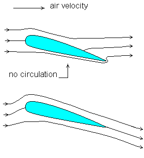
A wing (or airfoil or whatever) creates lift by taking advantage of a combination of the Bernoulli force and “angle of attack”.  By increasing angle of attack (tilting the nose up) the oncoming wind hits the bottom of the wing more, and pushes the plane up.  However, this force also increases drag substantially.  The Bernoulli force shows up when the air over the top of the wing is faster than the bottom, but it requires a bit of cleverness to get it to work.  Cleverness like the Kutta-Joukowski condition.

The Kutta-Joukowski condition: If air didn't flow faster over the top of the wing, then the air from the bottom would have to whip around the trailing edge with a very high acceleration. Too high, in fact. K-J assures that this singularity at the trailing edge doesn't show up.

When the Wright brothers built “the Flyer” (they were smart, not particularly creative) the engines available at the time were not powerful enough to lift themselves using only an angle of attack approach, so using a slick airfoil shape to take advantage of Bernoulli forces was essential to get off the ground.  Using the engines we have today (jets and whatnot) you could fly a brick, so long as the nose is pointed up.

So to actually answer the question; back in the day planes couldn’t fly upside-down.  But since then engines have become powerful enough to keep them in the air, despite the fact that by flying upside-down they’re being pushed toward the ground.  All they have to do is increase their angle of attack by pointing their nose up (or down, if you ask the pilot).

Posted in -- By the Physicist, Engineering, Physics | 21 Comments

Q: A flurry of blackhole questions!

Q: How much of the universe’s mass is currently in black holes?

Blackholes fall into two basic categories: stellar mass blackholes which have a mass of 3 to 30 Suns (give or take), and super-massive blackholes which usually have masses of more than 100,000 Suns.  Even in our own galaxy it’s essentially impossible to determine whether or not stellar mass blackholes are present.  I mean… they’re black, and they’re not heavy enough to throw around the nearby stars.  However, the supermassive blackholes do throw nearby stars around.  And that star-chucking property has allowed us to find that they have a mass of roughly 0.1% of the “bulge-mass” of the galaxies they sit in (the bulge is just the part of a galaxy that isn’t a disk).  So if I had to make a flying guestimate, I’d say that somewhere around 0.2% of the mass of any given galaxy is tied up in blackholes.

Q: Is there a graph of the number of black holes created since the big bang?

Probably.  Blackholes form from large stars, and large stars tend to have short lifetimes (a mere several million years).  So there should be a pretty sharp correlation between star formation rates and blackhole formation rates.  However, star formation rates are also notoriously difficult to measure.

Q: When was the first black hole created and when will the last one be?

Primordial Blackholes“, if they exist, would have formed almost instantly after the big bang.  If the Big Rip happens, then you can expect the last blackholes to form 50 million years before the end of the universe (give or take).  Otherwise, there’s no telling.

Q: How old will the universe be when black holes start to evaporate, if they even do?

Primordial blackholes should be popping right now.  The lightest stellar-mass blackholes (3 suns) won’t start evaporating until after the universe has cooled to below their Hawking temperature, which should be in about 13 billion years, when the universe is twice as old.  However, one age-of-the-universe is chump change compared to the 1069 years (about 10 billion trillion trillion trillion trillion times the age of the universe) it will take for the first stellar-mass blackholes to completely evaporate.

Q: Could all black holes evaporate away in a expanding cooling  universe?

Yup.

Q: What happens to the universe if all the back holes evaporate away?

No more blackholes?

Posted in -- By the Physicist, Astronomy, Physics | 11 Comments

Q: Why does going fast or being lower make time slow down?

Physicist: Back in the day, Galileo came up with the “Galilean Equivalence Principle” (GEP) which states that all the laws of physics work exactly the same, regardless of how fast you’re moving, or indeed whether or not you’re moving.  (Acceleration is a different story.  Acceleration screws everything up.)  What Einstein did was to tenaciously hold onto the GEP, regardless of what common sense and everyone around told him.  It turns out that the speed of light can be derived from a study of physical laws.  But if physics is the same for everybody, then the speed of light (hereafter “C”) must be the same for everybody.  The new principle, that the laws of physics are independent of velocity and that C is the same for everybody, is called the Einstein Equivalence Principle (EEP).

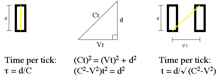
Moving faster makes time slow down: I’ve found that the best way to understand this is to actually do the calculation, then sit back and think about it.  Now, if a relativistic argument doesn’t hinge on the invariance of C, then it isn’t relativistic.  So ask yourself “What do the speed of light and time have to do with each other?”.  A good way to explore the connection is a “light clock”.  A light clock is a pair of mirrors, a fixed distance d apart, that bounce a photon back and forth and *clicks* at every bounce.  What follows is essentially the exact thought experiment that Einstein proposed to derive how time is affected by movement.

The proper time "τ" is how long it takes for the clock to tick if you're moving with it. The world time "t" is the time it takes for the clock to tick if you're moving with a relative velocity of V.

Let’s say Alice is holding a light clock, and Bob is watching her run by, while holding it, with speed V.  Alice is standing still (according to Alice), and the time, \tau, between ticks is easy to figure out: it’s just \tau = \frac{d}{C}.  From Bob’s perspective the photon in the clock doesn’t just travel up and down, it must also travel sideways, to keep up with Alice.  The additional sideways motion means that the photon has to cover a greater distance, and since it travels at a fixed speed (EEP y’all!) it must take more time.  The exact amount of time can be figured out by thinking about the distances involved.  Mix in a pinch of Pythagoras and Boom!: the time between ticks for Bob.  So Bob sees Alice’s clock ticking slower than Alice does.  You can easily reverse this experiment (just give Bob a clock), and you’ll see that Alice sees Bob’s clock running slow in exactly the same way.

It turns out that the really useful quantity here is the ratio: \frac{t}{\tau} = \frac{C}{d} \frac{d}{\sqrt{C^2 - V^2}} = \frac{C}{\sqrt{C^2 - V^2}} = \sqrt{\frac{C^2}{C^2-V^2}} = \sqrt{\frac{1}{1-\frac{V^2}{C^2}}} = \frac{1}{\sqrt{1-\frac{V^2}{C^2}}}.  This equation is called “gamma”.  It’s so important in relativity I’ll say it again: \gamma = \frac{1}{\sqrt{1-\frac{V^2}{C^2}}}.

It may seem at first glance that the different measurements are an illusion of some kind, like things in the distance looking smaller and slower, but unfortunately that’s not the case.  For Alice the light definitely travels a shorter distance, and the clock ticks faster.  For Bob the light really does travel a greater distance, and the clock ticks slower.  If you’re wondering why there’s no paradox, or want more details, then find yourself a book on relativity.  There are plenty.  Or look up Lorentz boosts.  (The very short answer is that position is also important.)

The lower the slower: Less commonly known, is that the lower you are in a gravity well, the slower time passes.  So someone on a mountain will age (very, very slightly) faster than someone in a valley.  This falls into the realm of general relativity, and the derivation is substantially more difficult.  Einstein crapped out special relativity in a few months, but it took him another 10 years to get general relativity figured out.  Here’s a good way to picture why (but not quite derive how) acceleration causes nearby points to experience time differently:

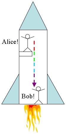
Redder light at the top, bluer light at the bottom.

Alice and Bob (again) are sitting at opposite ends of an accelerating rocket (that is to say; the rocket is on, so they’re speeding up).  Alice is sitting at the Apex (top) of the rocket and she’s shining a red light toward Bob at the Bottom of the rocket.  It takes some time (not much) for the light to get from the Apex of the rocket to the Bottom.  In that time Bob has had a chance to speed up a little, so by the time the light gets to him it will be a little bit blue-shifted.  Again, Alice sees red light at the Apex and Bob sees blue light at the Bottom.

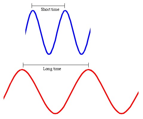
Counting the blue crests is faster than counting the red crests. However, since it's all the same light beam the number of crests has to be the same to everybody.

The time between wave crests for Bob are short, the time between wave crests for Alice are long.  Say for example that the blueshift increases the frequency by a factor of two, and Alice counts 10 crests per second.  Then Bob will count 20 crests per second (No new crests are being added in between the top and the bottom of the rocket).  Therefore, 2 seconds of Alice’s time happens in 1 second of Bob’s time.  Alice is moving through time faster.

Einstein’s insight (a way bigger jump than the EEP) was that gravitational acceleration and inertial acceleration are one and the same.  So the acceleration that pushes you down in a rocket does all the same things that the acceleration due to gravity does.  There’s no way to tell if the rocket is on and you’re flying through space, or if the rocket is off and you’re still on the launch pad.

It’s worth mentioning that the first time you read this it should be very difficult to understand.  Relativity = mind bending.

Posted in -- By the Physicist, Physics, Relativity | 109 Comments

Q: What’s so special about the Gaussian distribution (i.e. the normal distribution / bell curve)??

Physicist: A big part of what makes physicists slothful and attractive is a theorem called the “central limit theorem”.  In a nutshell it says that, even if you can’t describe how a single random thing happens, a whole mess of them together will act like a gaussian.  If you have a weighted die I won’t be able to tell you the probability of each individual number being rolled.  But (given the mean and variance) if you roll a couple dozen weighted dice and add them up I can tell you (with fairly small error) the probability of any sum, and the more dice the smaller the error.  Systems with lots of pieces added together show up all the time in practice, so knowing your way around a gaussian is well worth the trouble.

Gaussians also maximize entropy for a given energy (or other conserved quadratic quantity, energy is quadratic because E = \frac{1}{2} mv^2).  So if you have a bottle of gas at a given temperature (which fixes the total energy) you’ll find that the probability that a given particle is moving with a given velocity is given by a gaussian distribution.

From quantum mechanics, gaussians are the most “certain” wave functions.  The “Heisenberg uncertainty principle” states that for any wave function \Delta X \Delta P \ge \frac{\hbar}{2}, where \Delta X is the uncertainty in position and \Delta P is the uncertainty in momentum.  For a gaussian: \Delta X \Delta P = \frac{\hbar}{2}, the absolute minimum total uncertainty.

And much more generally, we know a lot about gaussians and there’s a lot of slick, easy math that works best on them.  So whenever you see a “bump” a good gut reaction is to pretend that it’s a “gaussian bump” just to make the math easier.  Sometimes this doesn’t work, but often it does or it points you in the right direction.


Mathematician: I’ll add a few more comments about the Gaussian distribution (also known as the normal distribution or bell curve) that the physicist didn’t explicitly touch on. First of all, while it is an extremely important distribution that arises a lot in real world applications, there are plenty of phenomenon that it does not model well. In particular, when the central limit theorem does not apply (i.e. our data points were not produced by taking a sum or average over samples drawn from more or less independent distributions) and we have no reason to believe our distribution should have maximum entropy, the normal distribution is the exception rather than the rule.

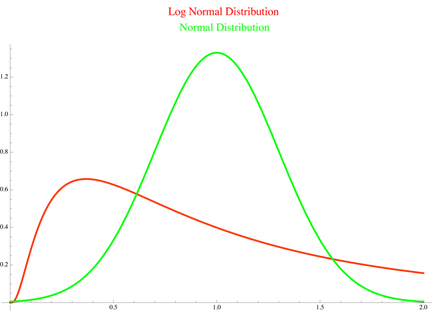
To give just one of many, many examples where non-normality arises: when we are dealing with a product (or geometric mean) of (essentially independent) random variables rather than a sum of them, we should expect that the resulting distribution will be approximately log-normal rather than normal (see image below). As it turns out, daily returns in the stock market are generally better modeled using a log-normal distribution rather than a normal distribution (perhaps this is the case because the most a stock can lose in one day is -100%, whereas the normal distribution assigns a positive probability to all real numbers). There are, of course, tons of other distributions that arise in real world problems that don’t look normal at all (e.g. the exponential distribution, Laplace distribution, Cauchy distribution, gamma distribution, and so on.)


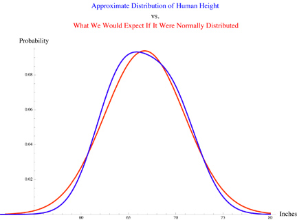
Human height provides an interesting case study, as we get distributions that are almost (but not quite) normally distributed. The heights of males (ignoring outliers) are close to being normal (perhaps height is the result of a sum of a number of nearly independent factors relating to genes, health, diet, etc.). On the other hand, the distribution of heights of people in general (i.e. both males and females together) looks more like the sum of two normal distributions (one for each gender), which in this case is like a slightly skewed normal distribution with a flattened top.


I’ll end with a couple more interesting facts about the normal distribution. In Fourier analysis we observe that, when it has an appropriate variance, the normal distribution is one of the eigenvectors of the Fourier transform operator. That is a fancy way of saying that the gaussian distribution represents its own frequency components. For instance, we have this nifty equation (relating a normal distribution to its Fourier transform):

e^{- \pi x^2}=\int_{-\infty}^{\infty} e^{- \pi s^2}e^{-2 \pi i s x} ds.

Note that the general equation for a (1 dimensional) Gaussian distribution (which tells us the likelihood of each value x) is

\frac{ e^{- \frac{(x-\mu)^2}{2 \sigma^2}} } {\sqrt{2 \pi \sigma^2}}

where \mu is the mean of the distribution, and \sigma is its standard deviation. Hence, the Fourier transform relation above deals with a normal distribution of mean 0 and standard deviation \frac{1}{\sqrt{2 \pi}}.

Another useful property to take note of relates to solving maximum likelihood problems (where we are looking for the parameters that make some data set as likely as possible). We generally end up solving these problems by trying to maximize something related to the log of the probability distribution under consideration. If we use a normal distribution, this takes the unusually simple form

\log{ \frac{ e^{- \frac{(x-\mu)^2}{2 \sigma^2}} } {\sqrt{2 \pi \sigma^2}} } = - \frac{(x-\mu)^2}{2 \sigma^2} - \frac{1}{2} \log(2 \pi \sigma^2)

which is often nice enough to allow for solutions that can be calculated exactly by hand. In particular, the fact that this function is quadratic in x makes it especially convenient, which is one reason that the Gaussian is commonly chosen in statistical modeling. In fact, the incredibly popular ordinary least squares regression technique can be thought of as finding the most likely line (or plane, or hyperplane) to fit a dataset, under the assumption that the data was generated by a linear equation with additive gaussian noise.

Posted in -- By the Mathematician, -- By the Physicist, Entropy/Information, Equations, Math, Probability, Quantum Theory | 11 Comments