Mathematician: Benford’s Law (sometimes called the Significant-Digit Law) states that when we gather numbers from many different types of random sources (e.g. the front pages of newspapers, tables of physical constants at the back of science textbooks, the heights of randomly selected animals picked from many different species, etc.), the probability that the leading digits (i.e. the left most non-zero digits) of one of these numbers will be  is approximately equal to
") .
.
That means the probability that a randomly selected number will have a leading digit of 1 is
 = 0.301")
which means it will happen about 30.1% of the time, whereas the probability that the first two leading digits will be 21 is given by
 = 0.020")
which means it will occur about 2.0% of the time. Note that if we were writing our numbers in a base  other than 10 (i.e. decimal) we would simply replace the
  in the formulas above with
  . Benford’s Law indicates that in base 10, the most likely leading digit for us to see is 1, the second most likely 2, the third most 3, the fourth most likely 4, and so on. But why should this be true, and to what sorts of sources of random numbers will it apply?
Some insight into Benford’s Law can be gleaned from the following mathematical fact: If there exists some universal distribution that describes the probability that numbers sampled from any source will have various leading digits, it must be the formula given above. The reason for this is because if such a formula works for all sources of data, then when we multiply all numbers produced by our source by any constant, the distribution of the likelihood of leading digits must not change. This is the property of “scale invariance”. Now notice that if we have a number whose leading digit is 5, 6, 7, 8, or 9, and we multiply that number by 2, the new leading digit will always be 1. But since this operation is not allowed to change the probability of leading digits, that means that the probability of having a leading digit of 1 must be the same as the probability of having a leading digit of any of 5, 6, 7, 8 or 9. This property is satisfied by the formula given above, since
 =")
 + log_{10}(1 +\frac{1}{6}) + log_{10}(1 + \frac{1}{7})")
 + log_{10}(1 + \frac{1}{9})")
Of course, there is nothing special about multiplying the numbers from our random source by 2, so a similar property must hold regardless of what we multiply our numbers by. As it turns out, the formula for Benford’s Law is the only formula such that the distribution does not change no matter what positive number we multiply the output of our random source by.
There is a problem with the preceding argument, however, since it has been empirically verified that not all data sources satisfy Benford’s Law in practice, so the existence of a universal law for leading digits seems to contradict the available evidence. On the other hand though, a great deal of data has been collected (e.g. by Benford himself) indicating that the law holds to pretty good accuracy for many different types of data sources. In fact, it seems that the law was first discovered due to a realization (by astronomer Simon Newcomb in 1881) that the pages of logarithm tables at the back of textbooks are not equally well worn. What was noticed was that the earlier tables (with numbers starting with the digit 1) tended to look rather dirtier than the later ones. So the question remains, how can we justify all of these empirical observations of the law in a more rigorous mathematical way?
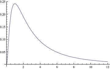
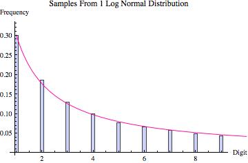
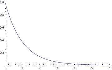
First of all, an important point to note is that when we sample values from some common probability distributions (like the exponential distribution and the log normal distribution) the leading digits that you get already come close to satisfying Benford’s Law (see the graphs at the bottom of the article). Hence, we should already expect the law to approximately hold in some real world scenarios. More importantly though, as was demonstrated by the probabilist Theodore Hill, if our process for sampling points actually involves sampling from multiple sources (which cover a variety of different scales, without favoring any scale in particular), and then group together all the points that we get from all of the sources, the distribution of leading digits will tend towards satisfying Benford’s Law. For the technical details and restrictions, check out Hill’s original 1996 paper.
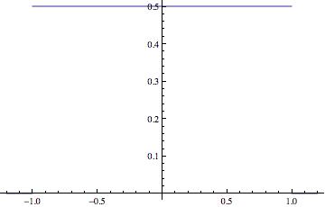
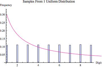
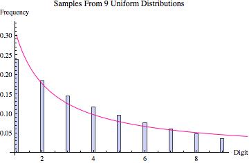
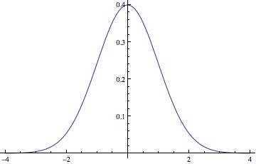
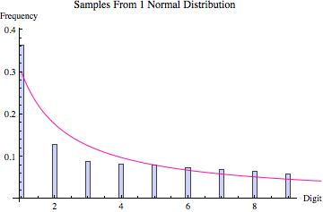
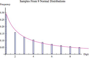
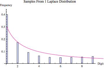
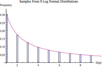
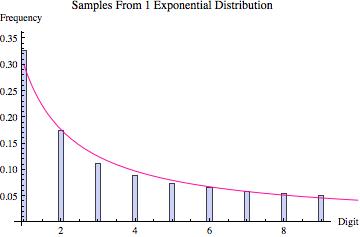
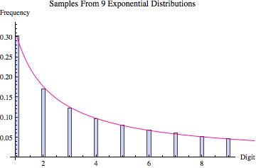
Perhaps the best way to quickly convince yourself that Hill’s result is true is to look at the graphs found below. Various probability distributions are shown (the first five that I happened to think of) together with the frequency of leading digits (from 1 to 9) that I got when sampling 100,000 points from that distribution (where the frequencies are depicted by the blue bars). For each, the pink line shows what we would expect to get if Benson’s Law held perfectly. As you can see, for some distributions we get a good fit (e.g. the exponential and log normal distributions) whereas for others the fit is poorer (e.g. the uniform, normal and laplace distributions). What the third graph in each table shows is the distribution of leading digits that we get when, instead of sampling just from one copy of each distribution, we sample from 9 different copies (with equal probability), each of which has a different variance (in most cases chosen to be proportional to the values 1 up to 9). Hence, what we are doing is sampling from multiple distributions each of which is the same except for a scaling factor, and then pooling those samples together, at which point we calculate the probability of the various leading digits (how often is 1 the first non-zero digit, how often is two the first non-zero digit, etc). The result in every case shown is that this leads to a distribution of leading digits that fits Benford’s Law quite well.
To conclude, when we are dealing with data that is combined from multiple sources such that those sources have no systematic bias in how they are scaled, we can expect that the distribution of leading digits will approximate Benford’s Law. This will tend to apply to sources like numbers pulled each day from the front page of a newspaper, because the values found in this way will come from all different distributions (some will represent oil prices, others real estate prices, others populations, and so on).
Besides just being generally bizarre and interesting, Benford’s Law has lately found some real world applications. For certain types of financial data where Benford’s Law applies, fraud has actually been detected by noting that results made up out of thin air will generally be non-random and will not satisfy the proper distribution of leading digits.
| Distribution |
Uniform |
| Probability Density Function |
|
| Distribution of Leading Digit Of Samples |
|
| Distribution of Leading Digit Taking Samples From 9 Such Distributions With Different Variances |
|
| Distribution |
Normal |
| Probability Density Function |
|
| Distribution of Leading Digit Of Samples |
|
| Distribution of Leading Digit Taking Samples From 9 Such Distributions With Different Variances |
|
| Distribution |
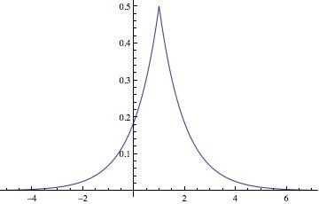
Laplace |
| Probability Density Function |
|
| Distribution of Leading Digit Of Samples |
|
| Distribution of Leading Digit Taking Samples From 9 Such Distributions With Different Variances |

|
| Distribution |
Log Normal |
| Probability Density Function |
|
| Distribution of Leading Digit Of Samples |
|
| Distribution of Leading Digit Taking Samples From 9 Such Distributions With Different Variances |
|
| Distribution |
Exponential |
| Probability Density Function |
|
| Distribution of Leading Digit Of Samples |
|
| Distribution of Leading Digit Taking Samples From 9 Such Distributions With Different Variances |
|