Physicist: A common refrain in quantum theory is “anything that can happen does”. Shockingly, and with total disregard for our own human experience, this seems to be true. When you consider what this means in the context of living and dying, a lot of weird, uncomfortable conclusions bubble up. In particular: if a situation can end with you either alive or dead, and every result literally does happen, then you will always experience a result where you live. No matter how ludicrously unlikely, if there’s a non-zero chance of surviving, then you always do. From your point of view, the world around you does whatever crazy contortions it must to ensure your continued point of view. “Quantum suicide” and “quantum immortality” get their name from this idea and that it may be impossible to die (from your own point of view), no matter how hard you try.
Quantum immortality is a philosophical thought experiment about what happens when you combine quantum many-state-ness with the anthropic principle and survivorship bias. It’s worth underscoring that this is a thought experiment, not advice. It’s an interesting idea, but I wouldn’t bet my life on it.
The anthropic principle says that whatever needed to happen in order for an observer to be observing, happened. For example, because you’re reading this, then (among other things) you must have access to the internet, speak English, live in an environment capable of supporting life, and were born rather than not born. For anyone/anything not reading this, none of those things may necessarily be true.
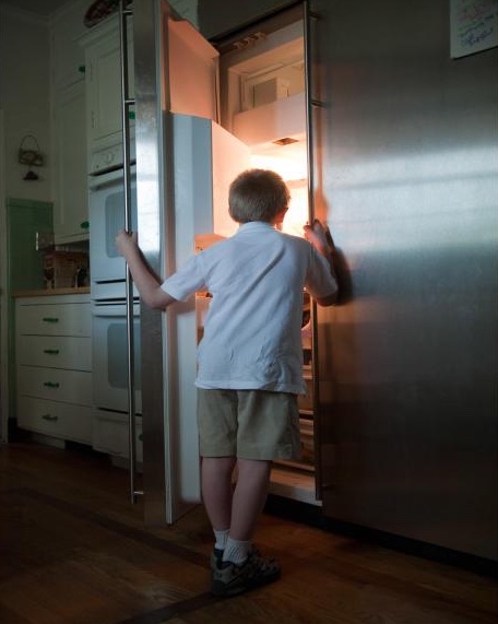
The anthropic principle helps explain why the refrigerator light seems to always be turned on. It’s set up to be on whenever you’re in a situation to see it.
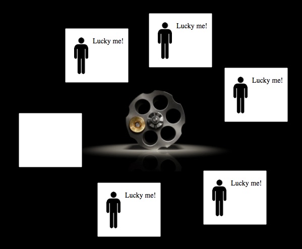
On it’s own, the anthropic principle is already pretty powerful. It is the governing principle behind why “you are here” signs are always accurate. It says that nobody ever regrets playing Russian Roulette, they only regret inviting their friends. And it explains why the Earth is capable of supporting introspective critters such as ourselves, despite all of the incredibly unlikely things that had to go right for that to happen. That last shouldn’t seem too surprising; if only one in a million planets can support life, where would you expect to find living things?
If every possible version of a given event does happen, then you will only (continue to) experience outcomes where you survive.
It’s the “quantum” that makes the quantum suicide thought experiment interesting. You’ll probably find a planet capable of supporting life in the universe, because there are a lot of opportunities (based on the other solar systems we can see) and there’s evidently a non-zero chance. What quantum theory does is change that “probably” to “definitely” if there’s ever a non-zero chance.
In classical physics (which is to say: when you just walk around and use your eyeballs), everything seems to be in a single state. Your coat is on one hook, not many. Your front door is open or closed, but not both. If you lose your keys, they’re someplace specific, even if you don’t happen to know where.
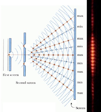
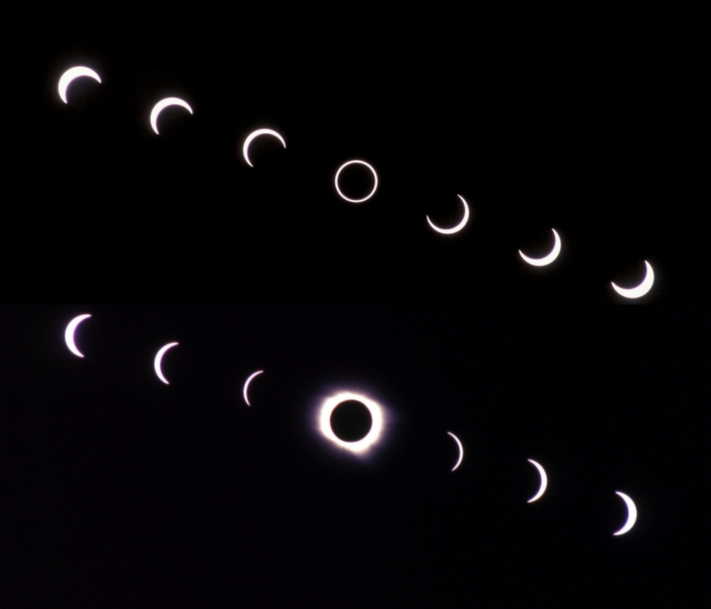
In quantum physics on the other hand, when we assume that things are in only one state our predictions fail. The most famous example of this is the double slit experiment, where coherent light is shined on a pair of slits (regular readers are no doubt sick of regularly reading about the vaunted double slit experiment). Instead of seeing two bars of light on the far side of the slits, we instead see “beats”; many bars of light corresponding to interference between every possible path through the two slits. The terrifying thing about the double slit experiment is that it continues to work even when the light intensity is turned down to just one photon at a time. If we assume that each photon goes through only one slit, then we expect to see a build up of photons in just two bars. The fact that we see many bars indicates that the photons go through both slits.
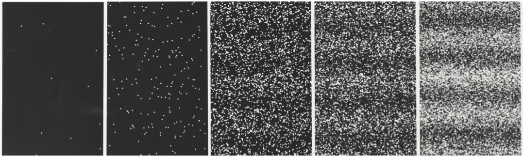
Even individually, when photons pass through the double slits they’ll hit a projection screen not in two bars, but in several, corresponding to wave interference between the two slits. In order to predict where a photon is likely to land, you have to take into account every possible path that it can take.
Other than being clearly weird, and simple enough for first-year physicists to do the math themselves, there is nothing special about the double slit experiment. The same “things can be in many states” idea applies across the board in quantum theory. It is the back bone of chemistry, particle interactions of all kinds, freaking everything.
And photons aren’t special either. You can do the double slit experiment with anything (as far as we know), it’s just that bigger things are harder to work with. The largest things to successfully demonstrate going through both slits are molecules of C284H190F320N4S12. That’s a modest 810 interconnected atoms! Our inability to demonstrate the quantumness of macroscopic things seems to be an engineering barrier rather than some undiscovered physical law. Every indication so far is that there’s no division between the “quantum world” and the “classical world”. Instead (like every other physical law), quantum laws seem to apply universally.
Notice that the refrain is “anything that can happen does” and not “everything happens”. Assuming the laws do apply on all scales, one of their more frustrating predictions is that the probability of observing yourself somewhere else is zero and the probability of observing two or more of yourselves is likewise zero (literally: wherever you go, there you are). These situations are impossible. Despite being in many states, none of your states directly interact with the others. Other quantum versions of yourself are like the bottom half of a Muppet; something you feel like you should be able to see, but there’s a good reason you never do.
This is not without precedent in science. For example, Newton’s laws simultaneously predict that 1) the Earth must be spinning and hurtling through space (based on how the other planets and stars move in the sky) and 2) that you’d never notice (because you’re hurtling along with the Earth). Arguably, this “it’s very weird, but it’s also really hard to notice” aspect of quantum mechanics is why it was discovered after bronze and the wheel.
The double slit experiment is so clean and easy to work with because you only have to worry about two states: the path that light can take through either slit. In reality the slits have some non-zero physical size, so there are many different paths photons can take through each. Those paths are all so similar that assuming they’re the same is good enough for an undergrad lab class. But if you want to nail down the exact pattern you see projected on the screen, you have to account for every possible path precisely. This is true whenever quantum theory applies (e.g., chemistry); counting the most likely quantum states buys you a decently accurate prediction, but the more states you take into account, the more accurate your prediction.
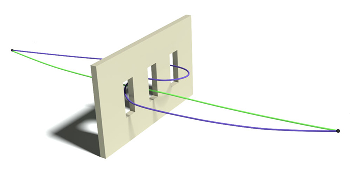
To perfectly predict quantum phenomena, we have to take into account every possible way an event can happen, even completely bizarre possibilities (such as this blue “non-classical path”). The less likely a path, the smaller its impact, but every path counts.
Low-probability states don’t add much, but they demonstrably add more than zero, so they must be physically real. A mountain and a pebble affect the world differently, but they’re “equally real”. So, assuming QM laws apply universally, every possible outcome of an event is physically realized and the fact that you can only experience situations where you’re alive means that you’ll be funneled into those realities where you continue to live.
There’s nothing ultimately special about life or death (unless you’re alive, and then it’s suddenly super important), they’re just more interesting to consider than, say, a quantum number generator that accidentally gives you sequential numbers forever. Quantum suicide makes some tricks a lot easier since the same quantumy arguments apply very broadly. For example, if a situation can end in either stubbing your toe or not, both results will occur. In some parallel histories, when you kick a brick barefoot you’ll miss. Still. What do you honestly think will happen if you try?
The central tenant of quantum immortality (that anything that can happen does) applies to everything and every combination of things, it’s just that we’re good at worrying about and keeping track of ourselves. There’s a vanishingly small probability that a Beanie Baby™ will “survive” intact for trillions of years (when it will have nearly doubled in value), so in some tiny set of the many possible futures it will. The fact that it doesn’t have a point of view means that it won’t be bothered one way or the other.
If there’s X chance that you’ll be walking around in a thousand years, then there’s a chance of about X2 that you and some other particular person will both be walking around. In other words, in some tiny fraction of possible futures you get to persist, and in a substantially more tiny (but still not quite zero) fraction you and Connor MacLeod are both alive. Until the gathering at least, after which there can be only one.

Connor MacLeod: immortal from the Scottish highlands or just an impossibly lucky cosplayer who accidentally hasn’t died?
So this gives us a way of testing out the completely insane idea of quantum immortality. If a bunch of us are accidentally alive in a thousand years, let’s all meet up and compare notes. We don’t need to bother agreeing on a meeting place or time, since quantum immortals should be used to relying on happenstance.
Quantum immortality is, almost by definition, a subjective experience. Clearly it’s possible to observe other people passing away (condolences everyone), but if quantum immortality is real, you’ll find out on your own. This has given rise to some clever science fiction, but not a lot of useful science fact. Point is: planning to live forever has not traditionally been an effective way to spend not-forever. I find myself alive and the improbable result of an endless string of nearly impossible coincidences, while on a world that may be unique in the universe. On the other hand, that’s everybody’s story and, not for nothing, don’t risk your life over some silly idea.
The “weaving photon” picture and a short summary of the experiment can be found here.
The fridge picture is from here.
MacLeod’s photo is from here.
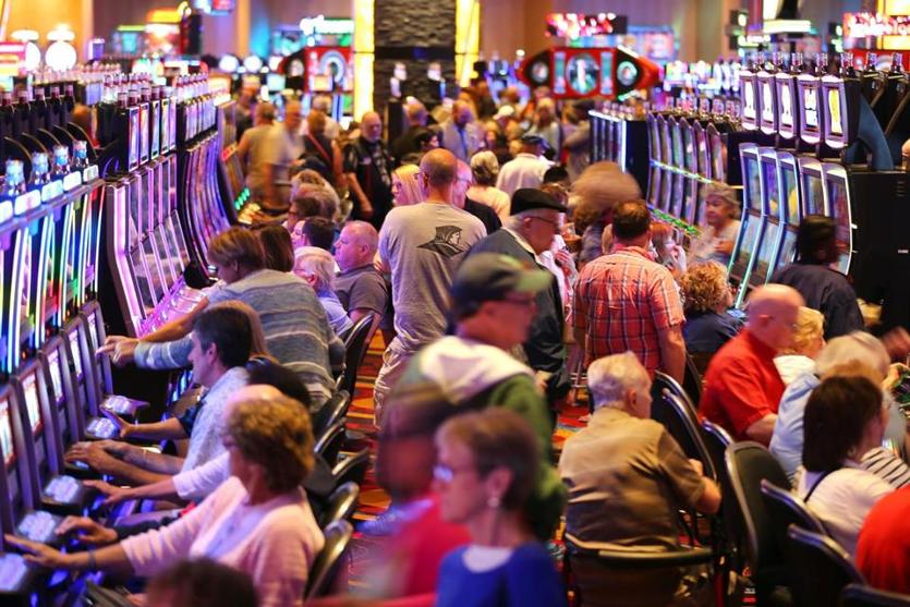
 (49.3%) probability of winning. Assuming you bet 1 “chip” (or whatever currency makes sense), then the first round you can either lose or gain 1 new chip. The amount of winnings you can expect (a mathematician would call this “the expected winnings”) is the probability of winning times how much you win, minus the probability you lose times how much you lose:
 (1)-\left(\frac{251}{495}\right)(1)\approx-0.014") . This is very intentionally negative, because on average you’re supposed lose.
. This is very intentionally negative, because on average you’re supposed lose. chips (you can add this up easily because it’s a
  chips. If you’ve got B chips in your pocket, then after
 \approx\log_2(B)") rounds you’ll be broke.
rounds you’ll be broke.=\log_2(1024)=\log_2\left(2^{10}\right)=10") rounds. For the pass line, the probability of losing ten games in a row and going broke is
rounds. For the pass line, the probability of losing ten games in a row and going broke is ^{10}\approx0.0011238") and the probability of winning before then and gaining one chip is
and the probability of winning before then and gaining one chip is  . So your expected winnings is
 1-\left(0.0011238\right)1023\approx-0.15") . Despite its cleverness, this system is actually worse than not being clever: if you just bet 1 chip ten times in a row, you can expect to lose about 0.14 chips (and only ten at most).
. Despite its cleverness, this system is actually worse than not being clever: if you just bet 1 chip ten times in a row, you can expect to lose about 0.14 chips (and only ten at most).
 chips, and if you win on the nth round, you’ll earn f times your last bet,
  .
. chips. This means that if you lose the first n-1 rounds and win on the nth, then your take-home winnings are
 =fm^{n-1}-\frac{m^{n-1}-1}{m-1}") .
.=q^{n-1}p") . So P(n) is the probability your ship will come in on the nth round and W(n) is how many chips you gain when it does. With those two equations in hand, you can find your expected winnings, E[W].
. So P(n) is the probability your ship will come in on the nth round and W(n) is how many chips you gain when it does. With those two equations in hand, you can find your expected winnings, E[W].![\begin{array}{rcl}E[W]&=&E\left[\left(f-\frac{1}{m-1}\right)m^{n-1}+\frac{1}{m-1}\right]\\[2mm]&=&\frac{1}{m-1}+\left(f-\frac{1}{m-1}\right)E\left[m^{n-1}\right]\\[2mm]&=&\frac{1}{m-1}+\left(f-\frac{1}{m-1}\right)\sum_{n=1}^\infty m^{n-1}P(n)\\[2mm]&=&\frac{1}{m-1}+\left(f-\frac{1}{m-1}\right)\sum_{n=1}^\infty m^{n-1}q^{n-1}p\\[2mm]&=&\frac{1}{m-1}+\left(f-\frac{1}{m-1}\right)p\sum_{n=1}^\infty (mq)^{n-1}\end{array}](https://s0.wp.com/latex.php?latex=%5Cbegin%7Barray%7D%7Brcl%7DE%5BW%5D%26%3D%26E%5Cleft%5B%5Cleft%28f-%5Cfrac%7B1%7D%7Bm-1%7D%5Cright%29m%5E%7Bn-1%7D%2B%5Cfrac%7B1%7D%7Bm-1%7D%5Cright%5D%5C%5C%5B2mm%5D%26%3D%26%5Cfrac%7B1%7D%7Bm-1%7D%2B%5Cleft%28f-%5Cfrac%7B1%7D%7Bm-1%7D%5Cright%29E%5Cleft%5Bm%5E%7Bn-1%7D%5Cright%5D%5C%5C%5B2mm%5D%26%3D%26%5Cfrac%7B1%7D%7Bm-1%7D%2B%5Cleft%28f-%5Cfrac%7B1%7D%7Bm-1%7D%5Cright%29%5Csum_%7Bn%3D1%7D%5E%5Cinfty+m%5E%7Bn-1%7DP%28n%29%5C%5C%5B2mm%5D%26%3D%26%5Cfrac%7B1%7D%7Bm-1%7D%2B%5Cleft%28f-%5Cfrac%7B1%7D%7Bm-1%7D%5Cright%29%5Csum_%7Bn%3D1%7D%5E%5Cinfty+m%5E%7Bn-1%7Dq%5E%7Bn-1%7Dp%5C%5C%5B2mm%5D%26%3D%26%5Cfrac%7B1%7D%7Bm-1%7D%2B%5Cleft%28f-%5Cfrac%7B1%7D%7Bm-1%7D%5Cright%29p%5Csum_%7Bn%3D1%7D%5E%5Cinfty+%28mq%29%5E%7Bn-1%7D%5Cend%7Barray%7D&bg=ffffff&fg=000000&s=0 "\begin{array}{rcl}E[W]&=&E\left[\left(f-\frac{1}{m-1}\right)m^{n-1}+\frac{1}{m-1}\right]\\[2mm]&=&\frac{1}{m-1}+\left(f-\frac{1}{m-1}\right)E\left[m^{n-1}\right]\\[2mm]&=&\frac{1}{m-1}+\left(f-\frac{1}{m-1}\right)\sum_{n=1}^\infty m^{n-1}P(n)\\[2mm]&=&\frac{1}{m-1}+\left(f-\frac{1}{m-1}\right)\sum_{n=1}^\infty m^{n-1}q^{n-1}p\\[2mm]&=&\frac{1}{m-1}+\left(f-\frac{1}{m-1}\right)p\sum_{n=1}^\infty (mq)^{n-1}\end{array}")
 , so if you can keep playing forever, then just by picking a large enough multiplier, m, the expected return is infinite. This is because the number of chips you get back after n rounds increases very exponentially with the number of rounds you play and there’s no chance of ever losing. It’s good to be richer than god.
 chips, which is all of them (because that’s how B is defined). The chance of losing all B rounds is
  .
.![\begin{array}{rl} E[W]=&\sum_{n=1}^BP(n)W(n)-q^B\frac{m^B-1}{m-1}\\[2mm] =&\sum_{n=1}^Bq^{n-1}p\left(\left(f-\frac{1}{m-1}\right)m^{n-1}+\frac{1}{m-1}\right)-\frac{(qm)^B-q^B}{m-1}\\[2mm] =&\sum_{n=1}^B\left(p\left(f-\frac{1}{m-1}\right)(qm)^{n-1}+\frac{p}{m-1}q^{n-1}\right)-\frac{(qm)^B-q^B}{m-1}\\[2mm] =&\left(pf-\frac{p}{m-1}\right)\sum_{n=1}^B(qm)^{n-1}+\frac{p}{m-1}\sum_{n=1}^Bq^{n-1}-\frac{(qm)^B-q^B}{m-1}\\[2mm] <&\left(q-\frac{p}{m-1}\right)\sum_{n=1}^B(qm)^{n-1}+\frac{p}{m-1}\sum_{n=1}^Bq^{n-1}-\frac{(qm)^B-q^B}{m-1}\\[2mm] =&\left(q+\frac{q-1}{m-1}\right)\sum_{n=1}^B(qm)^{n-1}-\frac{q-1}{m-1}\sum_{n=1}^Bq^{n-1}-\frac{(qm)^B-q^B}{m-1}\\[2mm] =&\left(\frac{qm-q+q-1}{m-1}\right)\sum_{n=1}^B(qm)^{n-1}-\frac{q-1}{m-1}\sum_{n=1}^Bq^{n-1}-\frac{(qm)^B-q^B}{m-1}\\[2mm] =&\left(\frac{qm-1}{m-1}\right)\sum_{n=1}^B(qm)^{n-1}-\frac{q-1}{m-1}\sum_{n=1}^Bq^{n-1}-\frac{(qm)^B-q^B}{m-1}\\[2mm] =&\left(\frac{qm-1}{m-1}\right)\frac{(qm)^B-1}{qm-1}-\frac{q-1}{m-1}\frac{q^B-1}{q-1}-\frac{(qm)^B-q^B}{m-1}\\[2mm] =&\frac{(qm)^B-1}{m-1}-\frac{q^B-1}{m-1}-\frac{(qm)^B-q^B}{m-1}\\[2mm] =&\frac{(qm)^B-1-q^B+1-(qm)^m+q^B}{m-1}\\[2mm] =&0 \end{array}](http://s0.wp.com/latex.php?latex=%5Cbegin%7Barray%7D%7Brl%7D++E%5BW%5D%3D%26%5Csum_%7Bn%3D1%7D%5EBP%28n%29W%28n%29-q%5EB%5Cfrac%7Bm%5EB-1%7D%7Bm-1%7D%5C%5C%5B2mm%5D++%3D%26%5Csum_%7Bn%3D1%7D%5EBq%5E%7Bn-1%7Dp%5Cleft%28%5Cleft%28f-%5Cfrac%7B1%7D%7Bm-1%7D%5Cright%29m%5E%7Bn-1%7D%2B%5Cfrac%7B1%7D%7Bm-1%7D%5Cright%29-%5Cfrac%7B%28qm%29%5EB-q%5EB%7D%7Bm-1%7D%5C%5C%5B2mm%5D++%3D%26%5Csum_%7Bn%3D1%7D%5EB%5Cleft%28p%5Cleft%28f-%5Cfrac%7B1%7D%7Bm-1%7D%5Cright%29%28qm%29%5E%7Bn-1%7D%2B%5Cfrac%7Bp%7D%7Bm-1%7Dq%5E%7Bn-1%7D%5Cright%29-%5Cfrac%7B%28qm%29%5EB-q%5EB%7D%7Bm-1%7D%5C%5C%5B2mm%5D++%3D%26%5Cleft%28pf-%5Cfrac%7Bp%7D%7Bm-1%7D%5Cright%29%5Csum_%7Bn%3D1%7D%5EB%28qm%29%5E%7Bn-1%7D%2B%5Cfrac%7Bp%7D%7Bm-1%7D%5Csum_%7Bn%3D1%7D%5EBq%5E%7Bn-1%7D-%5Cfrac%7B%28qm%29%5EB-q%5EB%7D%7Bm-1%7D%5C%5C%5B2mm%5D++%3C%26%5Cleft%28q-%5Cfrac%7Bp%7D%7Bm-1%7D%5Cright%29%5Csum_%7Bn%3D1%7D%5EB%28qm%29%5E%7Bn-1%7D%2B%5Cfrac%7Bp%7D%7Bm-1%7D%5Csum_%7Bn%3D1%7D%5EBq%5E%7Bn-1%7D-%5Cfrac%7B%28qm%29%5EB-q%5EB%7D%7Bm-1%7D%5C%5C%5B2mm%5D++%3D%26%5Cleft%28q%2B%5Cfrac%7Bq-1%7D%7Bm-1%7D%5Cright%29%5Csum_%7Bn%3D1%7D%5EB%28qm%29%5E%7Bn-1%7D-%5Cfrac%7Bq-1%7D%7Bm-1%7D%5Csum_%7Bn%3D1%7D%5EBq%5E%7Bn-1%7D-%5Cfrac%7B%28qm%29%5EB-q%5EB%7D%7Bm-1%7D%5C%5C%5B2mm%5D++%3D%26%5Cleft%28%5Cfrac%7Bqm-q%2Bq-1%7D%7Bm-1%7D%5Cright%29%5Csum_%7Bn%3D1%7D%5EB%28qm%29%5E%7Bn-1%7D-%5Cfrac%7Bq-1%7D%7Bm-1%7D%5Csum_%7Bn%3D1%7D%5EBq%5E%7Bn-1%7D-%5Cfrac%7B%28qm%29%5EB-q%5EB%7D%7Bm-1%7D%5C%5C%5B2mm%5D++%3D%26%5Cleft%28%5Cfrac%7Bqm-1%7D%7Bm-1%7D%5Cright%29%5Csum_%7Bn%3D1%7D%5EB%28qm%29%5E%7Bn-1%7D-%5Cfrac%7Bq-1%7D%7Bm-1%7D%5Csum_%7Bn%3D1%7D%5EBq%5E%7Bn-1%7D-%5Cfrac%7B%28qm%29%5EB-q%5EB%7D%7Bm-1%7D%5C%5C%5B2mm%5D++%3D%26%5Cleft%28%5Cfrac%7Bqm-1%7D%7Bm-1%7D%5Cright%29%5Cfrac%7B%28qm%29%5EB-1%7D%7Bqm-1%7D-%5Cfrac%7Bq-1%7D%7Bm-1%7D%5Cfrac%7Bq%5EB-1%7D%7Bq-1%7D-%5Cfrac%7B%28qm%29%5EB-q%5EB%7D%7Bm-1%7D%5C%5C%5B2mm%5D++%3D%26%5Cfrac%7B%28qm%29%5EB-1%7D%7Bm-1%7D-%5Cfrac%7Bq%5EB-1%7D%7Bm-1%7D-%5Cfrac%7B%28qm%29%5EB-q%5EB%7D%7Bm-1%7D%5C%5C%5B2mm%5D++%3D%26%5Cfrac%7B%28qm%29%5EB-1-q%5EB%2B1-%28qm%29%5Em%2Bq%5EB%7D%7Bm-1%7D%5C%5C%5B2mm%5D++%3D%260++%5Cend%7Barray%7D&bg=ffffff&fg=000&s=0 "\begin{array}{rl} E[W]=&\sum_{n=1}^BP(n)W(n)-q^B\frac{m^B-1}{m-1}\\[2mm] =&\sum_{n=1}^Bq^{n-1}p\left(\left(f-\frac{1}{m-1}\right)m^{n-1}+\frac{1}{m-1}\right)-\frac{(qm)^B-q^B}{m-1}\\[2mm] =&\sum_{n=1}^B\left(p\left(f-\frac{1}{m-1}\right)(qm)^{n-1}+\frac{p}{m-1}q^{n-1}\right)-\frac{(qm)^B-q^B}{m-1}\\[2mm] =&\left(pf-\frac{p}{m-1}\right)\sum_{n=1}^B(qm)^{n-1}+\frac{p}{m-1}\sum_{n=1}^Bq^{n-1}-\frac{(qm)^B-q^B}{m-1}\\[2mm] <&\left(q-\frac{p}{m-1}\right)\sum_{n=1}^B(qm)^{n-1}+\frac{p}{m-1}\sum_{n=1}^Bq^{n-1}-\frac{(qm)^B-q^B}{m-1}\\[2mm] =&\left(q+\frac{q-1}{m-1}\right)\sum_{n=1}^B(qm)^{n-1}-\frac{q-1}{m-1}\sum_{n=1}^Bq^{n-1}-\frac{(qm)^B-q^B}{m-1}\\[2mm] =&\left(\frac{qm-q+q-1}{m-1}\right)\sum_{n=1}^B(qm)^{n-1}-\frac{q-1}{m-1}\sum_{n=1}^Bq^{n-1}-\frac{(qm)^B-q^B}{m-1}\\[2mm] =&\left(\frac{qm-1}{m-1}\right)\sum_{n=1}^B(qm)^{n-1}-\frac{q-1}{m-1}\sum_{n=1}^Bq^{n-1}-\frac{(qm)^B-q^B}{m-1}\\[2mm] =&\left(\frac{qm-1}{m-1}\right)\frac{(qm)^B-1}{qm-1}-\frac{q-1}{m-1}\frac{q^B-1}{q-1}-\frac{(qm)^B-q^B}{m-1}\\[2mm] =&\frac{(qm)^B-1}{m-1}-\frac{q^B-1}{m-1}-\frac{(qm)^B-q^B}{m-1}\\[2mm] =&\frac{(qm)^B-1-q^B+1-(qm)^m+q^B}{m-1}\\[2mm] =&0 \end{array}")


 passes through) and horizontally polarized (
 is stopped). So for a vertical (or horizontal) filter the measurement basis is
  .
. , is a superposition of both
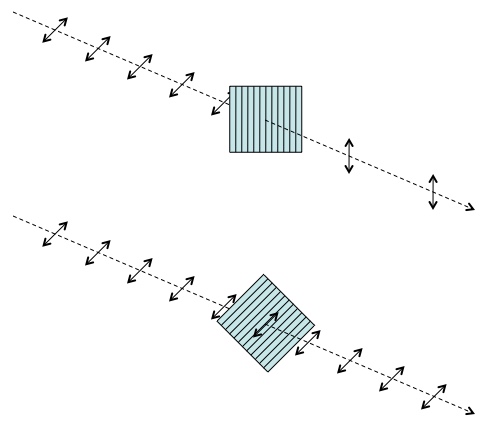
 basis. If the incoming state is one of those diagonal states, then the diagonal filter will determine which. When you measure diagonal photons with a similarly diagonal filter, they always pass through and there’s no collapse to either of the vertical/horizontal states.
") . The subscript “a” means “owned by Alice”. This notation says that if Alice measures her photon in the
. The subscript “a” means “owned by Alice”. This notation says that if Alice measures her photon in the  chance of either result according to the
 ") . Both of these diagonal states produce random results in the
. Both of these diagonal states produce random results in the  basis, but produce definite results in the
  basis.
") and
and ") , so the vertical and horizontal states are superpositions of the diagonal states and therefore produce random results in the diagonal basis. For each of these states (or any other for that matter), there is a measurement basis where they give definite results.
, so the vertical and horizontal states are superpositions of the diagonal states and therefore produce random results in the diagonal basis. For each of these states (or any other for that matter), there is a measurement basis where they give definite results.") . This notation says that if either Alice or Bob do a measurement in the
. This notation says that if either Alice or Bob do a measurement in the ![\begin{array}{ll} &\frac{1}{\sqrt{2}}\left(|\rightarrow\rangle_a|\rightarrow\rangle_b+|\uparrow\rangle_a|\uparrow\rangle_b\right)\\[2mm] =&\frac{1}{\sqrt{2}}\left(\frac{1}{\sqrt{2}}\left(|\nearrow\rangle_a-|\nwarrow\rangle_a\right)\frac{1}{\sqrt{2}}\left(|\nearrow\rangle_b-|\nwarrow\rangle_b\right)+\frac{1}{\sqrt{2}}\left(|\nearrow\rangle_a+|\nwarrow\rangle_a\right)\frac{1}{\sqrt{2}}\left(|\nearrow\rangle_b+|\nwarrow\rangle_b\right)\right)\\[2mm] =&\frac{1}{2\sqrt{2}}\left(\left(|\nearrow\rangle_a-|\nwarrow\rangle_a\right)\left(|\nearrow\rangle_b-|\nwarrow\rangle_b\right)+\left(|\nearrow\rangle_a+|\nwarrow\rangle_a\right)\left(|\nearrow\rangle_b+|\nwarrow\rangle_b\right)\right)\\[2mm] =&\frac{1}{2\sqrt{2}}\left(\begin{array}{l}|\nearrow\rangle_a|\nearrow\rangle_b-|\nearrow\rangle_a|\nwarrow\rangle_b-|\nwarrow\rangle_a|\nearrow\rangle_b+|\nwarrow\rangle_a|\nwarrow\rangle_b\\+|\nearrow\rangle_a|\nearrow\rangle_b+|\nearrow\rangle_a|\nwarrow\rangle_b+|\nwarrow\rangle_a|\nearrow\rangle_b+|\nwarrow\rangle_a|\nwarrow\rangle_b\end{array}\right)\\[2mm] =&\frac{1}{2\sqrt{2}}\left(2|\nearrow\rangle_a|\nearrow\rangle_b+2|\nwarrow\rangle_a|\nwarrow\rangle_b\right)\\[2mm] =&\frac{1}{\sqrt{2}}\left(|\nearrow\rangle_a|\nearrow\rangle_b+|\nwarrow\rangle_a|\nwarrow\rangle_b\right)\\[2mm] \end{array}](http://s0.wp.com/latex.php?latex=%5Cbegin%7Barray%7D%7Bll%7D++%26%5Cfrac%7B1%7D%7B%5Csqrt%7B2%7D%7D%5Cleft%28%7C%5Crightarrow%5Crangle_a%7C%5Crightarrow%5Crangle_b%2B%7C%5Cuparrow%5Crangle_a%7C%5Cuparrow%5Crangle_b%5Cright%29%5C%5C%5B2mm%5D++%3D%26%5Cfrac%7B1%7D%7B%5Csqrt%7B2%7D%7D%5Cleft%28%5Cfrac%7B1%7D%7B%5Csqrt%7B2%7D%7D%5Cleft%28%7C%5Cnearrow%5Crangle_a-%7C%5Cnwarrow%5Crangle_a%5Cright%29%5Cfrac%7B1%7D%7B%5Csqrt%7B2%7D%7D%5Cleft%28%7C%5Cnearrow%5Crangle_b-%7C%5Cnwarrow%5Crangle_b%5Cright%29%2B%5Cfrac%7B1%7D%7B%5Csqrt%7B2%7D%7D%5Cleft%28%7C%5Cnearrow%5Crangle_a%2B%7C%5Cnwarrow%5Crangle_a%5Cright%29%5Cfrac%7B1%7D%7B%5Csqrt%7B2%7D%7D%5Cleft%28%7C%5Cnearrow%5Crangle_b%2B%7C%5Cnwarrow%5Crangle_b%5Cright%29%5Cright%29%5C%5C%5B2mm%5D++%3D%26%5Cfrac%7B1%7D%7B2%5Csqrt%7B2%7D%7D%5Cleft%28%5Cleft%28%7C%5Cnearrow%5Crangle_a-%7C%5Cnwarrow%5Crangle_a%5Cright%29%5Cleft%28%7C%5Cnearrow%5Crangle_b-%7C%5Cnwarrow%5Crangle_b%5Cright%29%2B%5Cleft%28%7C%5Cnearrow%5Crangle_a%2B%7C%5Cnwarrow%5Crangle_a%5Cright%29%5Cleft%28%7C%5Cnearrow%5Crangle_b%2B%7C%5Cnwarrow%5Crangle_b%5Cright%29%5Cright%29%5C%5C%5B2mm%5D++%3D%26%5Cfrac%7B1%7D%7B2%5Csqrt%7B2%7D%7D%5Cleft%28%5Cbegin%7Barray%7D%7Bl%7D%7C%5Cnearrow%5Crangle_a%7C%5Cnearrow%5Crangle_b-%7C%5Cnearrow%5Crangle_a%7C%5Cnwarrow%5Crangle_b-%7C%5Cnwarrow%5Crangle_a%7C%5Cnearrow%5Crangle_b%2B%7C%5Cnwarrow%5Crangle_a%7C%5Cnwarrow%5Crangle_b%5C%5C%2B%7C%5Cnearrow%5Crangle_a%7C%5Cnearrow%5Crangle_b%2B%7C%5Cnearrow%5Crangle_a%7C%5Cnwarrow%5Crangle_b%2B%7C%5Cnwarrow%5Crangle_a%7C%5Cnearrow%5Crangle_b%2B%7C%5Cnwarrow%5Crangle_a%7C%5Cnwarrow%5Crangle_b%5Cend%7Barray%7D%5Cright%29%5C%5C%5B2mm%5D++%3D%26%5Cfrac%7B1%7D%7B2%5Csqrt%7B2%7D%7D%5Cleft%282%7C%5Cnearrow%5Crangle_a%7C%5Cnearrow%5Crangle_b%2B2%7C%5Cnwarrow%5Crangle_a%7C%5Cnwarrow%5Crangle_b%5Cright%29%5C%5C%5B2mm%5D++%3D%26%5Cfrac%7B1%7D%7B%5Csqrt%7B2%7D%7D%5Cleft%28%7C%5Cnearrow%5Crangle_a%7C%5Cnearrow%5Crangle_b%2B%7C%5Cnwarrow%5Crangle_a%7C%5Cnwarrow%5Crangle_b%5Cright%29%5C%5C%5B2mm%5D++%5Cend%7Barray%7D&bg=ffffff&fg=000&s=0 "\begin{array}{ll} &\frac{1}{\sqrt{2}}\left(|\rightarrow\rangle_a|\rightarrow\rangle_b+|\uparrow\rangle_a|\uparrow\rangle_b\right)\\[2mm] =&\frac{1}{\sqrt{2}}\left(\frac{1}{\sqrt{2}}\left(|\nearrow\rangle_a-|\nwarrow\rangle_a\right)\frac{1}{\sqrt{2}}\left(|\nearrow\rangle_b-|\nwarrow\rangle_b\right)+\frac{1}{\sqrt{2}}\left(|\nearrow\rangle_a+|\nwarrow\rangle_a\right)\frac{1}{\sqrt{2}}\left(|\nearrow\rangle_b+|\nwarrow\rangle_b\right)\right)\\[2mm] =&\frac{1}{2\sqrt{2}}\left(\left(|\nearrow\rangle_a-|\nwarrow\rangle_a\right)\left(|\nearrow\rangle_b-|\nwarrow\rangle_b\right)+\left(|\nearrow\rangle_a+|\nwarrow\rangle_a\right)\left(|\nearrow\rangle_b+|\nwarrow\rangle_b\right)\right)\\[2mm] =&\frac{1}{2\sqrt{2}}\left(\begin{array}{l}|\nearrow\rangle_a|\nearrow\rangle_b-|\nearrow\rangle_a|\nwarrow\rangle_b-|\nwarrow\rangle_a|\nearrow\rangle_b+|\nwarrow\rangle_a|\nwarrow\rangle_b\\+|\nearrow\rangle_a|\nearrow\rangle_b+|\nearrow\rangle_a|\nwarrow\rangle_b+|\nwarrow\rangle_a|\nearrow\rangle_b+|\nwarrow\rangle_a|\nwarrow\rangle_b\end{array}\right)\\[2mm] =&\frac{1}{2\sqrt{2}}\left(2|\nearrow\rangle_a|\nearrow\rangle_b+2|\nwarrow\rangle_a|\nwarrow\rangle_b\right)\\[2mm] =&\frac{1}{\sqrt{2}}\left(|\nearrow\rangle_a|\nearrow\rangle_b+|\nwarrow\rangle_a|\nwarrow\rangle_b\right)\\[2mm] \end{array}")

\\|1\rangle&\to&\frac{1}{\sqrt{2}}\left(|0\rangle-|1\rangle\right)\end{array}")
![\begin{array}{rl}&\frac{1}{\sqrt{2}}\left(|0\rangle_a|0\rangle_b+|1\rangle_a|1\rangle_b\right)\\[2mm]\xrightarrow{CNot}&\frac{1}{\sqrt{2}}\left(|0\rangle_a|0\rangle_b+|1\rangle_a|0\rangle_b\right)\\[2mm]=&\frac{1}{\sqrt{2}}\left(|0\rangle_a+|1\rangle_a\right)|0\rangle_b\\[2mm]\xrightarrow{H}&|0\rangle_a|0\rangle_b\end{array}](https://s0.wp.com/latex.php?latex=%5Cbegin%7Barray%7D%7Brl%7D%26%5Cfrac%7B1%7D%7B%5Csqrt%7B2%7D%7D%5Cleft%28%7C0%5Crangle_a%7C0%5Crangle_b%2B%7C1%5Crangle_a%7C1%5Crangle_b%5Cright%29%5C%5C%5B2mm%5D%5Cxrightarrow%7BCNot%7D%26%5Cfrac%7B1%7D%7B%5Csqrt%7B2%7D%7D%5Cleft%28%7C0%5Crangle_a%7C0%5Crangle_b%2B%7C1%5Crangle_a%7C0%5Crangle_b%5Cright%29%5C%5C%5B2mm%5D%3D%26%5Cfrac%7B1%7D%7B%5Csqrt%7B2%7D%7D%5Cleft%28%7C0%5Crangle_a%2B%7C1%5Crangle_a%5Cright%29%7C0%5Crangle_b%5C%5C%5B2mm%5D%5Cxrightarrow%7BH%7D%26%7C0%5Crangle_a%7C0%5Crangle_b%5Cend%7Barray%7D&bg=ffffff&fg=000000&s=0 "\begin{array}{rl}&\frac{1}{\sqrt{2}}\left(|0\rangle_a|0\rangle_b+|1\rangle_a|1\rangle_b\right)\\[2mm]\xrightarrow{CNot}&\frac{1}{\sqrt{2}}\left(|0\rangle_a|0\rangle_b+|1\rangle_a|0\rangle_b\right)\\[2mm]=&\frac{1}{\sqrt{2}}\left(|0\rangle_a+|1\rangle_a\right)|0\rangle_b\\[2mm]\xrightarrow{H}&|0\rangle_a|0\rangle_b\end{array}")
![\begin{array}{rcl}\frac{1}{\sqrt{2}}\left(|0\rangle_a|0\rangle_b+|1\rangle_a|1\rangle_b\right)&\to&|0\rangle_a|0\rangle_b\\[2mm]\frac{1}{\sqrt{2}}\left(|0\rangle_a|0\rangle_b-|1\rangle_a|1\rangle_b\right)&\to&|1\rangle_a|0\rangle_b\\[2mm]\frac{1}{\sqrt{2}}\left(|0\rangle_a|1\rangle_b+|1\rangle_a|0\rangle_b\right)&\to&|0\rangle_a|1\rangle_b\\[2mm]\frac{1}{\sqrt{2}}\left(|0\rangle_a|1\rangle_b-|1\rangle_a|0\rangle_b\right)&\to&|1\rangle_a|1\rangle_b\end{array}](https://s0.wp.com/latex.php?latex=%5Cbegin%7Barray%7D%7Brcl%7D%5Cfrac%7B1%7D%7B%5Csqrt%7B2%7D%7D%5Cleft%28%7C0%5Crangle_a%7C0%5Crangle_b%2B%7C1%5Crangle_a%7C1%5Crangle_b%5Cright%29%26%5Cto%26%7C0%5Crangle_a%7C0%5Crangle_b%5C%5C%5B2mm%5D%5Cfrac%7B1%7D%7B%5Csqrt%7B2%7D%7D%5Cleft%28%7C0%5Crangle_a%7C0%5Crangle_b-%7C1%5Crangle_a%7C1%5Crangle_b%5Cright%29%26%5Cto%26%7C1%5Crangle_a%7C0%5Crangle_b%5C%5C%5B2mm%5D%5Cfrac%7B1%7D%7B%5Csqrt%7B2%7D%7D%5Cleft%28%7C0%5Crangle_a%7C1%5Crangle_b%2B%7C1%5Crangle_a%7C0%5Crangle_b%5Cright%29%26%5Cto%26%7C0%5Crangle_a%7C1%5Crangle_b%5C%5C%5B2mm%5D%5Cfrac%7B1%7D%7B%5Csqrt%7B2%7D%7D%5Cleft%28%7C0%5Crangle_a%7C1%5Crangle_b-%7C1%5Crangle_a%7C0%5Crangle_b%5Cright%29%26%5Cto%26%7C1%5Crangle_a%7C1%5Crangle_b%5Cend%7Barray%7D&bg=ffffff&fg=000000&s=0 "\begin{array}{rcl}\frac{1}{\sqrt{2}}\left(|0\rangle_a|0\rangle_b+|1\rangle_a|1\rangle_b\right)&\to&|0\rangle_a|0\rangle_b\\[2mm]\frac{1}{\sqrt{2}}\left(|0\rangle_a|0\rangle_b-|1\rangle_a|1\rangle_b\right)&\to&|1\rangle_a|0\rangle_b\\[2mm]\frac{1}{\sqrt{2}}\left(|0\rangle_a|1\rangle_b+|1\rangle_a|0\rangle_b\right)&\to&|0\rangle_a|1\rangle_b\\[2mm]\frac{1}{\sqrt{2}}\left(|0\rangle_a|1\rangle_b-|1\rangle_a|0\rangle_b\right)&\to&|1\rangle_a|1\rangle_b\end{array}")


(5.97\times10^{24}kg)}{3.85\times 10^8m}}(0.04m)=1.49\times10^{24}\frac{m^2kg}{s}")
(5N)(1year)=6.07\times10^{16}\frac{m^2kg}{s}")


